SIGN Excel Function

Last Updated :

21 Aug, 2024

Blog Author :

Edited by :

Reviewed by :

Table Of Contents

SIGN Function in Excel

The SIGN function in Excel is a Maths/Trig function that gives us this result. The SIGN function returns the sign (-1, 0, or +1) of the supplied numerical argument. The SIGN formula in Excel can be used by typing the keyword: =SIGN( and providing the number as input.

For example, suppose we have a dataset of sales of a product for two years in cells A1(80,000) and B1(50,000). Now, we want to see if there is an increase in the figure compared to last year. In such a scenario, we can use the following SIGN formula:

=SIGN(A1-B1)

=+1.

SIGN Function in Excel

Syntax

Arguments

the number: It is the number to get the sign for.

The input number can be any number entered directly or in the form of any mathematical operation or cell reference.

Output:

The SIGN formula in Excel has only three results: +1, 0, and -1.

If the number exceeds zero, the Excel SIGN formula will return 1.
If the number equals zero, the SIGN formula in Excel will return 0.
If the number is less than zero, the SIGN formula in Excel will return -1.

If the supplied number argument is non-numeric, the Excel SIGN function will return #VALUE! Error.

SIGN Excel Function Video

How to Use the SIGN Function in Excel? (with Examples)

Example #1

Suppose you have the final balance figures for seven departments for 2016 and 2017, as shown below.

Departments	2016	2017
Department A	10000	12000
Department B	-1890	-2000
Department C	250000	320000
Department D	80000	60000
Department E	-50000	-40000
Department F	-1000	2500
Department G	12000	12500

Some departments are running in debt, and some are giving good returns. Now, you want to see if there is an increase in the figure compared to last year. To do so, you can use the following SIGN formula for the first one.

=SIGN(D4 - C4)

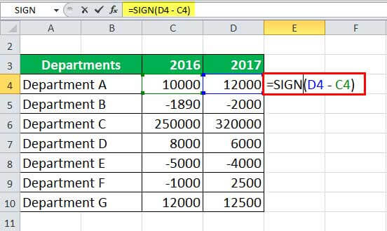
It will return +1. The argument to the SIGN function is a value returned from other functions.

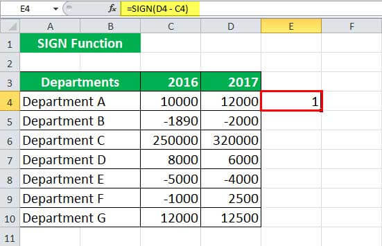
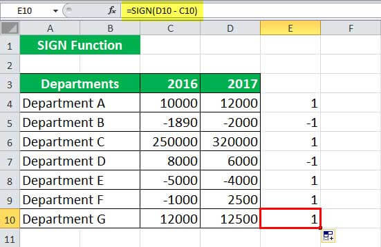
Drag it to get the value for the rest of the cells.

Example #2

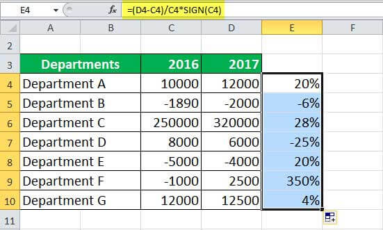
In the above example, you may also want to calculate the percentage increase in excel concerning the previous year.

For that, you can use the following SIGN formula:

=(D4 - C4)/C4 * SIGN(C4)

Drag it to the rest of the cells.

If the balance for 2016 is zero, the function will give an error. Alternatively, we may use the following SIGN formula to avoid the error:

=IFERROR((D4 - C4) / C4 * SIGN(C4), 0)

To get the overall percentage of increase or decrease, you can use the following formula:

(SUM(D4:D10) – SUM(C4:C10)) / SUM(C4:C10) * SIGN(SUM(C4:C10))

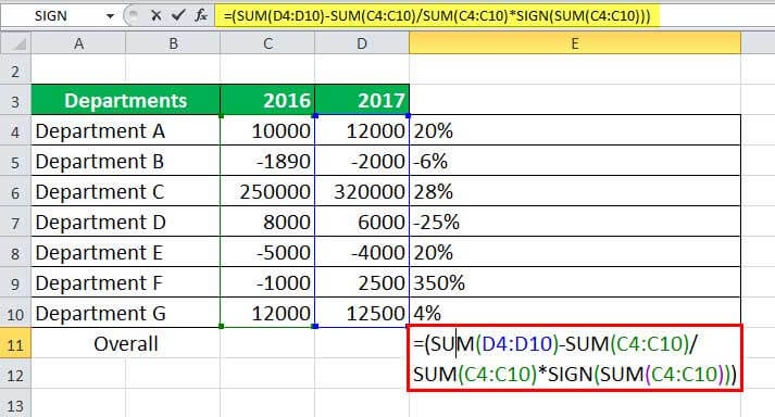
SUM(D4:D10) will give the net balance including all departments for 2017

SUM(C4:C10) will give the net balance including all departments for 2016

SUM(D4:D10) – SUM(C4:C10) will give the net gain or loss, including all departments.

(SUM(D4:D10) – SUM(C4:C10)) / SUM(C4:C10) * SIGN(SUM(C4:C10)) will give the percentage gain or loss

Example #3

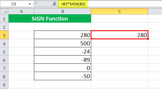
Suppose you have a list of numbers in B3:B8, as shown below.

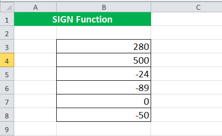
Now, you want to change the negative number's sign to positive.

You may use the following formula:

=B3 * SIGN(B3)

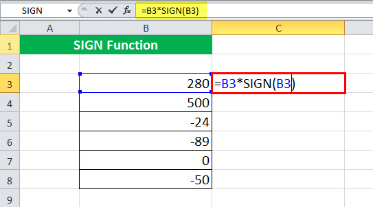
If the B3 is negative, SIGN(B3) is -1, and B3 * SIGN(B3) will be negative * negative, which will return positive.

If the B3 is positive, SIGN(B3) is +1, and B3 * SIGN(B3) will be positive * positive, which will return positive.

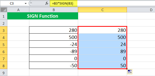
It will return to 280.

Drag it to get the values for the rest of the numbers.

Example #4

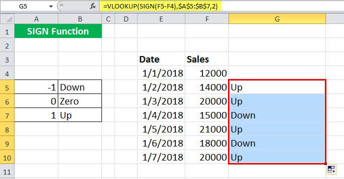
Suppose you have your monthly sales in F4:F10 and want to find out if your sales are going up and down.

To do so, you can use the following formula:

=VLOOKUP(SIGN(F5 – F4), A5:B7, 2)

A5:B7 contains the information on the up, zero, and down.

The SIGN function will compare the current and previous month's sales using the SIGN function. The VLOOKUP Excel function will pull the information from the VLOOKUP table and return whether the sales are going up, zero, or down.

Drag it to the rest of the cells.

Example #5

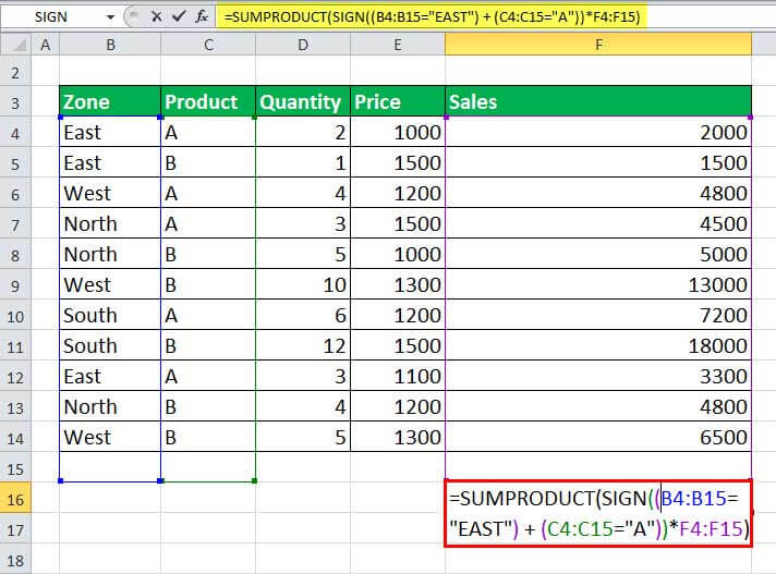
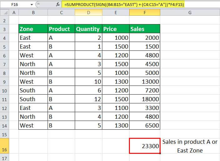
Suppose you have sales data from four zones: East, West, North, and South for products A and B, as shown below.

Zone	Product	Quantity	Price	Sales
East	A	2	1000	2000
East	B	1	1500	1500
West	A	4	1200	4800
North	A	3	1500	4500
North	B	5	1000	5000
West	B	10	1300	13000
South	A	6	1200	7200
South	B	12	1500	18000
East	A	3	1100	3300
North	B	4	1200	4800
West	B	5	1300	6500

Now, you want the total sales for product A or East zone.

It can be calculated as:

=SUMPRODUCT(SIGN((B4:B15 = “EAST”) + (C4:C15 = “A”)) * F4:F15)

Let us see the above SIGN function in detail.

B4:B15 = “EAST”

It will give 1 if it is “EAST” else it will return 0. It will return {1, 1, 0, 0, 0, 0, 0, 0, 1, 0, 0}

C4:C15 = “A”

It will give 1 if it is “A” else it will return 0. It will return {1, 0, 1, 1, 0, 0, 1, 0, 1, 0, 0}

(B4:B15 = “EAST”) + (C4:C15 = “A”)

It will return sum the two and {0, 1, 2}. It will return {2, 2, 1, 1, 0, 0, 1, 0, 2, 0, 0}

SIGN((B4:B15 = “EAST”) + (C4:C15 = “A”))

It will then return {0, 1} here since there is no negative number. It will return {1, 1, 1, 1, 0, 0, 1, 0, 1, 0, 0}.

SUMPRODUCT(SIGN((B4:B15 = “EAST”) + (C4:C15 = “A”)) * F4:F15)

It will first take the product of the two matrix {1, 1, 1, 1, 0, 0, 1, 0, 1, 0, 0} and {2000, 1500, 4800, 4500, 5000, 13000, 7200, 18000, 3300, 4800, 6500} which will return {2000, 1500, 4800, 4500, 0, 0, 7200, 0, 3300, 0, 0}, and then sum it.

It will finally return 23,300.

Similarly, to calculate the product sales for East or West zones, you may use the following SIGN formula:

=SUMPRODUCT(SIGN((B4:B15 = “EAST”) + (B4:B15 = “WEST”)) * F4:F15)

For product A in East zone:

=SUMPRODUCT(SIGN((B4:B15 = “EAST”) * (C4:C15 = “A”)) * F4:F15)