Top 4 Must Know Investment Banking Charts (Free Download Template included)

Investment Banking Charts refers to the different graphs, charts, financial models or the valuation model which helps the Investment banking firms in making the different analysis used for its functioning and the different types of investment banking charts include PE chart, PE band chart, Football field graph, and scenario graph, etc.

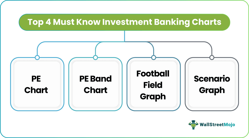
Investment Banking Charts – Football Field & PE Band Charts

I think the greatest gift of Dan Bricklin (“father” of the electronic spreadsheet) and Bill Gates to Investment Banking Mankind is the Excel spreadsheet software that allows the analyst to not only create rock star financial and valuation models but also help present their analysis in some awesome pictorial format (graphs).

With this, I thought, why not a tutorial on the most popular Investment Banking, Graphs vs. chartsGraphs Vs. ChartsGraphs are mostly a numerical representation of data which shows the relation of change in numbers to how one number is affecting or changing another. However, charts are the visual representation of categories that may or may not be related to each other.read more. In this article, I will discuss the following set of graphs –

1. PE Chart
2. PE Band Chart
3. Football Field Graph
4. Scenario Graph (my favorite)

Download the Spreadsheet templates for all the graphs here

You are free to use this image on your website, templates etc, Please provide us with an attribution linkHow to Provide Attribution?Article Link to be Hyperlinked
For eg:
Source: Top 4 Must Know Investment Banking Charts (Free Download Template included) (wallstreetmojo.com)

# 1 – PE Chart

This PE ratioPE RatioThe price to earnings (PE) ratio measures the relative value of the corporate stocks, i.e., whether it is undervalued or overvalued. It is calculated as the proportion of the current price per share to the earnings per share. read more is, in essence, a payback calculation: it states how many years’ earnings it will take for the investor to recover the price paid for the shares. PE (price to earnings) charts help us to understand the valuation multiple over time. Other things being equal, when comparing the price of two stocks in the same sector, the investor should prefer the one with the lowest PE. If you are new to PE ratiosPE RatiosThe price to earnings (PE) ratio measures the relative value of the corporate stocks, i.e., whether it is undervalued or overvalued. It is calculated as the proportion of the current price per share to the earnings per share. read more, you may refer to this valuation primer article on Relative Valuations.

What is a PE Chart

PE chart helps the investors visualize the trading valuation multiple of Stock or Index over a period of time. For example, the below PE graph of a company named Foodland Farsi is depicted over a period of March’02 until March’07.

Interpretation of PE Charts

• Historically Foodland Farsi has traded a an average PE multiple of 8.6x
• The standard deviation of the PE multiple signifies the volatility of the PE multiple.
• We note that Foodland Farsi has traded within the range formed by the Upper (defined as Average PE + 1 Std Dev = 12.2x) and the Lower (Average PE – 1 Std Dev  = 4.9x)
• We note that the PE multiple for the period after June ’06 has crossed the upper standard deviation line signifying higher valuation multiple.

Why is it useful?

• This chart is fairly useful because this provides the historical valuation details in a quick and easy format.
• You may take not more than 30 seconds to interpret such a graph.

Dataset for PE Chart

Let us now prepare the PE chart as provided above. Please download the PE Chart dataset here. The dataset includes the following –

• Date
• Historical Stock Prices
• EPS estimate (forward) – Please note that this data may not be available in the public forum. You may use Bloomberg, Factset, Factiva (all are paid versions) to get access to such data

Building a PE Chart

Step 1 – Calculate the PE Ratio

Since we already know the Price of the Stock and the Forward EPS, calculate the PE ratio of the stock for each date.

Step 2 – Calculate the Standard Deviation of PE

Calculating Standard Deviation is fairly easy in Excel. You can use the formula STDDEV to calculate the standard deviation of the stock. Do not forget to use absolute referencesUse Absolute ReferencesAbsolute reference in excel is a type of cell reference in which the cells being referred to do not change, as they did in relative reference. By pressing f4, we can create a formula for absolute referencing.read more so as to display the same standard deviations across the dates.

Step 3 – Calculate the Average PE

Calculate the Average PE of the stock using the formula AVERAGE and also use absolute references as the average of the data should remain constant across all the dates.

Step 4 – Calculate the UPPER and the LOWER range.

Calculate the UPPER and the LOWER range by using the following formula

• UPPER = Average PE + Standard Deviation
• LOWER = Average PE – Standard Deviation

Step 5 – Plot the Graph using the following data –

1. Forward PE
2. Average PE
3. UPPER
4. LOWER

Step 6 – Format the Graph

This is very important as formatting can really win if you can highlight the important areas and make it more intuitive to comprehend.

Like the PE charts, you can also make Price to Book Value Chart (P/BV), PEGPEGThe PEG ratio compares the P/E ratio of a company to its expected rate of growth. A PEG ratio of 1.0 or lower, on average, indicates that a stock is undervalued. A PEG ratio greater than 1.0 indicates that a stock is overvalued.read more Graph, Price to Sales, or Price to Cashflow Charts.

#2 – PE Band Chart

What is PE Band Chart?

Like the PE Ratio Graph, PE Band is also computed from the historical PE ratios for each individual stock/Index. The line plotted from the average highest PE will form the upper PE Band, whereas the average lowest PE will form the lower PE Band. The middle PE Band will be derived from the mean of the Upper and Lower Band.

Interpretation of PE Band Chart

The above chart can be interpreted as follows

• Currently, the Price Line (colored in GREEN) is touching the Maximum PE Band Line of 20.2x. This implies that the stock is trading at its maximum PE and maybe overvalued!
• The upper band reflects the Historical Maximum Price of the stock if the stock would have traded at its Maximum PE. For example, If we trace back the Maximum PE Band Line till March’02, we find that the stock would have traded at Rs600/- if the PE during that period would be 20.2x
• Also, we note that the stock has touched the lowest PE Band of 5.0x many times in the last 5 years period. It denotes an ideal opportunity to buy the stock.

Why is PE Band Chart Useful?

• The advantage of the PE Band is its consideration for both the fundamental factor (i.e., profitability) and the historical trading pattern of a stock.
• The use of PE Band is especially meaningful for listed companies, which have profitable track records.
• For a stock with stable earnings, its price tends to move within the PE Band. In other words, the stock price in one extreme tends to move to the other extreme within the Band.
• Also, note that the PE Band Chart is different from the PE ratio graph as we note that the Y-axis represents the price of the stock rather than the PE multiple.
• This PE Band Chart is effective because this graph is able to denote both the PE Bands (valuation) and the corresponding Prices. Along with the PE ratio graphs, this makes a case for taking a valuation call on stocks.

PE Band Chart Data set

The PE Band Chart Data Set is no different from the one that we used earlier. In fact, it is the same! We require the following –

• Historical Stock Prices
• Dates
• Forward EPS

 Building a PE Band Chart

Step 1 – Calculate the Forward PEForward PEForward PE ratio uses the forecasted earnings per share of the company over the next 12 months for calculating the price-earnings ratio. Forward PE ratio formula = Price per share/Projected earnings per share read more for the Historical Dataset

Step 2 – Calculate the average, maximum, and the minimum of the PE ratios

Step 3 – Find the Implied Prices using the following formula

Calculate the implied prices using the formula below

• Price  (corresponding to Average) = Average PE x (Historical EPS)
• Price  (corresponding to Maximum) = Maximum PE x (Historical EPS)
• Price  (corresponding to Minimum) = Minimum PE x (Historical EPS)

Step 4 – Plot the graph using the following

• Stock Price
• Implied Average Price
• Implied Maximum Price
• Implied Minimum Price

Step 5 – Format the Graph :-)

You can make Band Charts for another set of valuation multiples like EV/EBITDA EV/EBITDAEV to EBITDA is the ratio between enterprise value and earnings before interest, taxes, depreciation, and amortization that helps the investor in the valuation of the company at a very subtle level by allowing the investor to compare a specific company to the peer company in the industry as a whole, or other comparative industries.read more (Enterprise Value to EBITDA), P/CF, etc

#3 – Football Field Graph

What is Football Field Chart?

Sometimes it is easier for us to represent the data in floating columns or bars in which columns (or bars) float spanning a region from minimum to the maximum values. Below is a sample Football Field column chart.

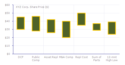
Interpretation of the Football Field Chart (above)

• The data represents fair valuation (Price/Share) of the company under different assumptions and valuation methodsValuation MethodsDiscounted cash flow, comparable company analysis, comparable transaction comps, asset valuation, and sum of parts are the five methods for valuing a company.read more.
• Using DCF, the valuation of the firm comes out to be $30/share (pessimistic case) and $45 under (most optimistic case).
• The highest fair valuation of the company is $50/share when using the Replacement Cost methodReplacement Cost MethodReplacement Cost is the capital amount required to replace the current asset with a similar one at the present market rate. Usually, assets replacement occurs when their repair & maintenance charges surge beyond a reasonable level. read more of valuation.
• However, the lowest fair valuation comes out to be $20/share when using M&A Transaction Comp valuation.

Data for Football Field Chart

Let us assume that you have been provided with the following set of data. You want to represent the below data in the best possible graphical format.

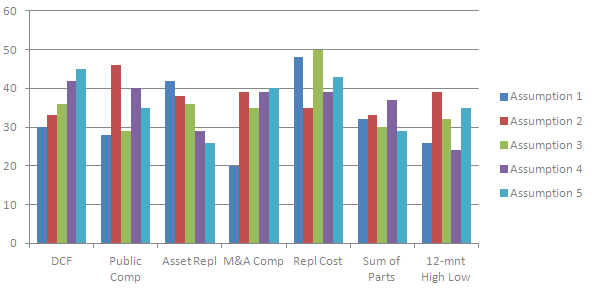
There can be different ways of making graphs on such data; however, they may not provide great insights when we make a regular line graph or the bar graphs. Below are the representation (poor) of these regular graphs –

Line Graph

The problem with this representation is that it is very difficult to interpret this data.

Column Graph

Again the same problem that it is very difficult to interpret such data.

With this, it is now easy to understand that the solution lies in making the floating column or the bar chart in excel.

Building a Football Field Chart

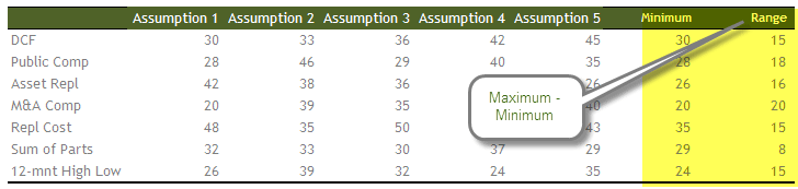
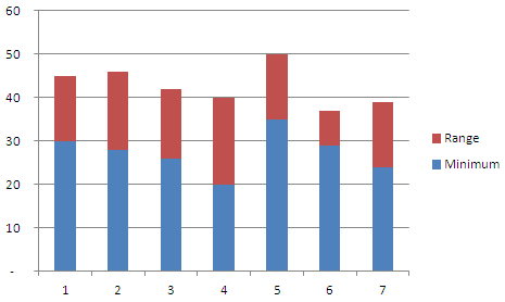
Step 1 – Create the Two series with Minimum and Range.

The first series represents the minimum, and the second represents the range (maximum-minimum). Please see below the two series on which we create our graph.

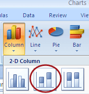
Step 2 – Choose Stacked Column Chart

The secret to making the floating chart is to use the column chart in excelColumn Chart In ExcelColumn chart is used to represent data in vertical columns. The height of the column represents the value for the specific data series in a chart, the column chart represents the comparison in the form of column from left to right.read more in an effective way by selecting the “stacked column chart in excelStacked Column Chart In ExcelA stacked column chart in Excel is a column chart in which multiple series of data representations of various categories are stacked over each other. The stacked series are vertical, and comparing multiple data series is easy, but as the number of data series increases, so does the complexity of representation.read more” using two series.

You will get the below chart.

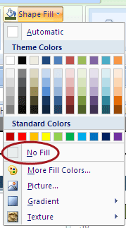
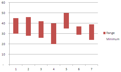
Step 3 – Make the “minimum” columns Invisible!

Select the minimum column bars (blue color) and from the top menu, change the color to “No Fill.”

With this, you will get the graph below.

Step 4 – Format the graph and make it awesome!

• Change the x-axis to reflect the valuation methodology.
• Remove the Legends on the right-hand side (Range and Minimum)
• Change the color of the bars to suit your color taste (please don’t make the columns as pink; it’s Investment Banking, you know!)

# 4 – Scenario Graphs

What are Scenario Graphs?

Sometimes It is important for us to accept the fact that understand that valuation is not a very scientific approach. It depends on assumptions and scenarios. While we value a stock, you may make a different set of assumptions while preparing a financial model – projecting income statement, balance sheetBalance SheetA balance sheet is one of the financial statements of a company that presents the shareholders' equity, liabilities, and assets of the company at a specific point in time. It is based on the accounting equation that states that the sum of the total liabilities and the owner's capital equals the total assets of the company.read more, and cash flows. While it is important for us to take the most expected case while we do the valuation, it is equally important to show the impact of different cases like what if the tax rates go down or what if the production moves up more than expected, etc. These scenarios can be easily built using Financial Models.

You can use the following financial models for your reference –

• Alibaba IPO Financial Model 
• Box IPO Financial Model

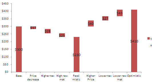
Please see below a sample Scenario Graph –

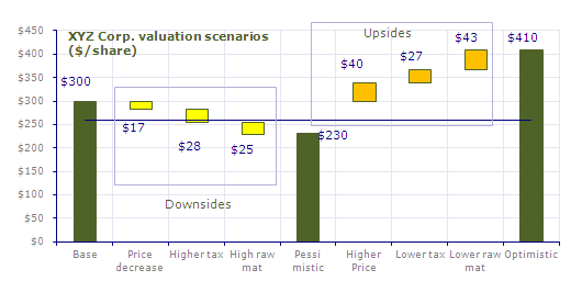
Interpretation of Scenario Graph

• We note from above that the base case valuation for the stock XYZ is $300
• The scenario graphs provide us with additional inputs on downsides with respect to the following.
  • If the price of the product decreases, then the fair price of the stock would go down by $17.
  • If corporate taxesCorporate TaxesCorporate tax is a tax levied by the government on the profits earned by a company at a fixed rate each year and is calculated in accordance with specific tax regulations.read more are higher, then the fair price of the stock would move further down by another $28
  • If raw material prices move up, then fair prices of the stock would move down even more by another $25.
  • If we consider all the pessimistic cases (an event when all three negative events happen together), then the fair valuation of the stock would drop to $230 per share.
• Likewise, you can find the additional inputs on the upsides – If we consider all the optimistic cases (Higher prices, higher taxes, and lower raw material costs), the fair price of the stock would move up to $410 per share.

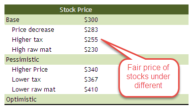
Dataset for the Scenario Graphs

The dataset required for this graph is shown below. The table below is arrived at after inputting new assumptions in your Financial Model and recalculating the fair share price.

Building a Scenario Graph

We will assume that you already have the data like the one above. With this, let us look at the steps involved to build the Scenario Graphs –

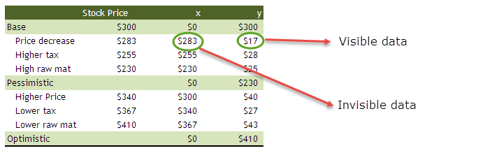
Step 1 – Add two columns X and Y in the data-set (tricky and most important)

• This graph builds on the Football Field Graph (#3) that we earlier made.
• In this, we again use the Column Stacked Graph, where Y data gets stacked over the X data.
• In addition to this, we make the X dataset as invisible so that we get the floating Y dataset.
• For example, if you closely observe the scenario graph – downside scenario – Price decrease shows a floating visible data of $17 (Y data), and immediately below this dataset is the invisible $283 (X Data).

Step 2 – The completed X and Y dataset should look something like below.

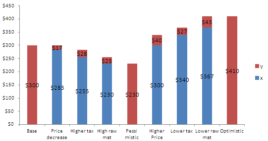
Step 3 – Prepare the Column Stacked Graph on the two dataset X and Y

Please note that we are not preparing the chart on the original set of data. We are preparing the chart on the converted dataset (X and Y)

 Step 4 – Make the X dataset hidden.

Hide the X dataset by selecting the columns and choosing “No Fill” from the Formatting options in the menu

Step 5 – Format the Graph, and be awesome!

Conclusions

As we note above that there can be a different graphical representation of stock valuation. The primary reason we use such graphs is to comply with save time for the clients and make the research report or pitch book a time saving and effective document. You will find the four types of valuation graphs in a majority of the tier-1 brokerage firm research reports. I had worked earlier at JPMorgan as an equity research analyst and found the Football field graph and Scenario graph to be the most useful representation for clients. You can use these in Ratio analysisRatio AnalysisRatio analysis is the quantitative interpretation of the company's financial performance. It provides valuable information about the organization's profitability, solvency, operational efficiency and liquidity positions as represented by the financial statements.read more Graphs too.

Recommended Articles

• Investment Banking Operations Course
• Investment Banking Downloads | Free Templates, Models
• Investment Banking in Atlanta
• Investment Banking Interview Questions with Answer
• Top Investment Banking in Malaysia

What’s Next?

If you learned something new or enjoyed the post, please leave a comment below. Let me know what you think. Many thanks, and take care.