Part of our Formatting in Excel guide
What Is Shade Alternate Rows In Excel?
Shade Alternate Rows in Excel is a feature where in a given dataset, we can highlight alternate rows using the shading methods, as the name suggests. In this feature, we can either shade alternate rows or the required rows.
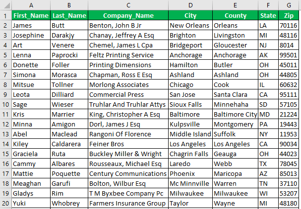
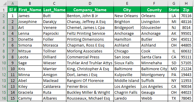
For example, we have the following dataset. One common method to Shade Alternate Rows is using the conditional formatting technique.
Once we apply “Conditional Formatting” on the above data, we get the following output, with alternate rows shaded or highlighted. We can also change the shading color as desired.

Key Takeaways
- We can highlight or shade the desired rows, here, the alternate rows either from the first or second row and so on, using the Shade Alternate Rows in Excel methods.
- Using the “Conditional Formatting” method, we can highlight the rows by creating a New Rule and inserting MOD() and ROWS() formulas.
- The conditional formatting feature works based on logical results, “TRUE” or “FALSE”, and highlights the rows accordingly.
- We can also use VBA code to Shade Alternate Rows and execute the code using the VBA Macro.
How To Shade Alternate Rows In Excel?
We can Shade Alternate Rows in Excel using the following methods, namely,
We will use the data given below to understand the shading methods.
Method #1 – Without Using Helper Column
We will first use the Conditional Formatting method to Shade Alternate Rows without the helper column.
The steps to shade every alternate row are as follows:
Select the entire data (without heading).
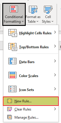
Go to Conditional Formatting, and choose “New Rule”.

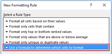
In the next window, choose “Use a formula to determine which cells to format”.

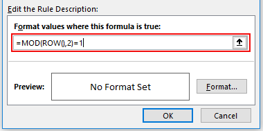
In the conditional formatting field enter the formula =MOD(ROW(),2)=1

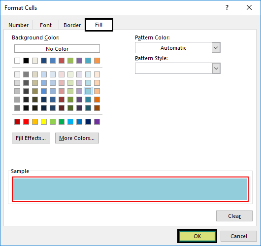
Click on the Format tab to choose the formatting color.

Now, it will open up the format cells window. Choose the tab “FILL”, and choose the color as per your wish.

Click Ok to see the shades in an alternative row.


We get the above output due to the MOD() and ROW() formulas.
- The MOD Excel function is the formula to get the remainder value when dividing one number by the other. For example, MOD (3, 2) will return 1 as the remainder, i.e., when we divide number 3 by number 2, we will get the remainder value as 1.
- The ROW() function will return the respective row number, and the same row number will be divided by 2. Again, if the remainder equals number 1, that row will be highlighted or shaded by the chosen color.
Method #2 – Using Helper Column
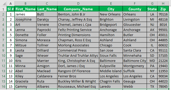
We can Shade Alternate Rows in Excel by inserting the helper column of serial numbers.
- For this, we must first insert a “Serial Number” column like the below one, i.e., column A.
- Now select the data except the helper column.
- Again, open “Conditional Formatting” and choose the same method, but this time we will change only the formula. Insert the formula as =ISODD(A2) and make it absolute.
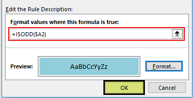
- Click OK. We will get an alternative shaded row.
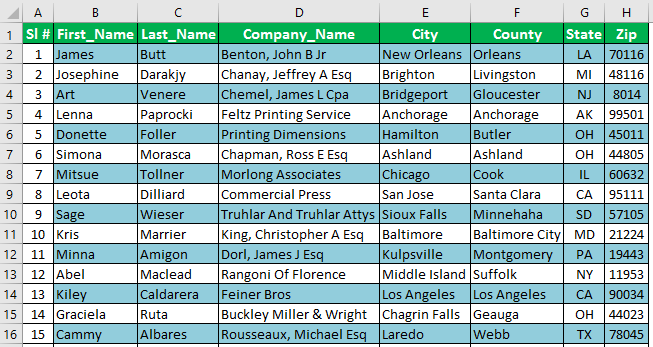
The output shown above is slightly different from the Method 1 output because, in Method 1, the alternate shaded rows started from the second Row, whereas in Method 2, the shading starts from the first row of the data, i.e., the row itself has been highlighted.
Method #3 – Using VBA Coding
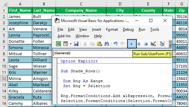
You can use the below VBA code to shade every alternative row. Use the below code to Shade Alternate Rows in Excel.
Code:
Sub Shade_Rows() Dim Rng As Range Set Rng = Selection Rng.FormatConditions.Add xlExpression, Formula1:=”=MOD(ROW(),2)=1″ Selection.FormatConditions(Selection.FormatConditions.Count).SetFirstPriority With Selection.FormatConditions(1).Interior .PatternColorIndex = xlAutomatic .ThemeColor = xlThemeColorAccent5 .TintAndShade = 0.399945066682943 End With Selection.FormatConditions(1).StopIfTrue = False End Sub
First, select the cell range to be shaded, and then run the macro.
Important Things To Note
- We can also shade every third, fourth, or fifth row, alternative rows, and so on. We must change the divisor value in the MOD function from 2 to 3.
- The ISODD and ISEVEN functions are useful with the helper column of serial numbers.
Frequently Asked Questions (FAQs)
Why to Shade Alternate Rows in Excel?
The Shade Alternate Rows help users highlight the required rows. It helps to present the data in an organized and presentable way which is easy to comprehend.
Name the different methods To Shade Alternate Rows In Excel.
We can Shade Alternate Rows in Excel using the following methods, namely,
a. Without Using any Helper Column.
b. Using Helper Column, and
c. Using VBA Coding.
Where is the Conditional Formatting option to shade alternate rows?
First, choose the dataset – select the “Home” tab – go to the “Styles” group – click the “Conditional Formatting” drop-down – select the “New Rule” option, as shown below.
Now, set the rules or conditions as discussed in the Method 2 section.
Any other simple method to shade rows in Excel?
We have another alternative method other than the Conditional Formatting with or without Header Columns, VBA Code, etc.
First, choose the dataset – select the “Home” tab – go to the “Styles” group – click the “Format as Table” drop-down, as shown below.
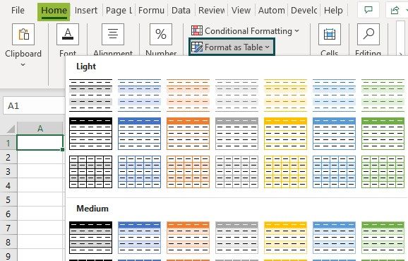
Here, we have various table styles under the “Light, Medium and Dark” categories. Choose the desired format which has alternate shading styles, and the dataset will automatically get updated with highlighted rows.
Recommended Articles
This article is a guide to Shade Alternate Rows in Excel. Here, we learn to shade rows, helper columns, conditional formatting, example & downloadable template. You may learn more about Excel from the following articles: –