Part of our Formatting in Excel guide
How to Split a Cell in Excel?
Let us consider some examples to understand the splitting of cells with the help of thetext to columns wizard.
Example #1–Split by “Delimited” Option
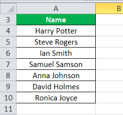
The following table shows the full names of seven people. We want to split the first and the last name into separate columns. Use the “delimited” option of the text to columns wizard.
The steps to split cells in excel with the help of the delimiter character are listed as follows:
- Select the cell range A3:A10, which is to be split. The same is shown in the following image.

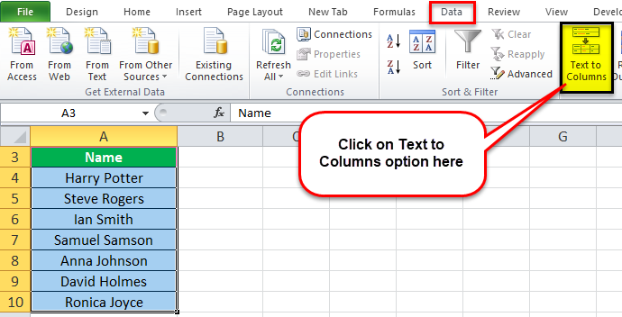
- In the Data tab, click the “text to columns” option under the “data tools” group.

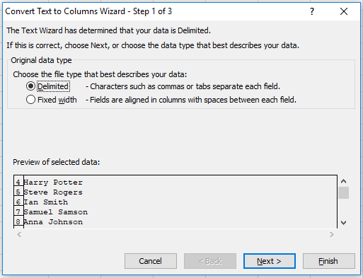
- The “convert text to columns wizard” dialog box appears, as shown in the following image.

- Choose the “delimited” option, which is selected by default. This option helps separate the data strings based on a particular delimiter character. Click “next.”
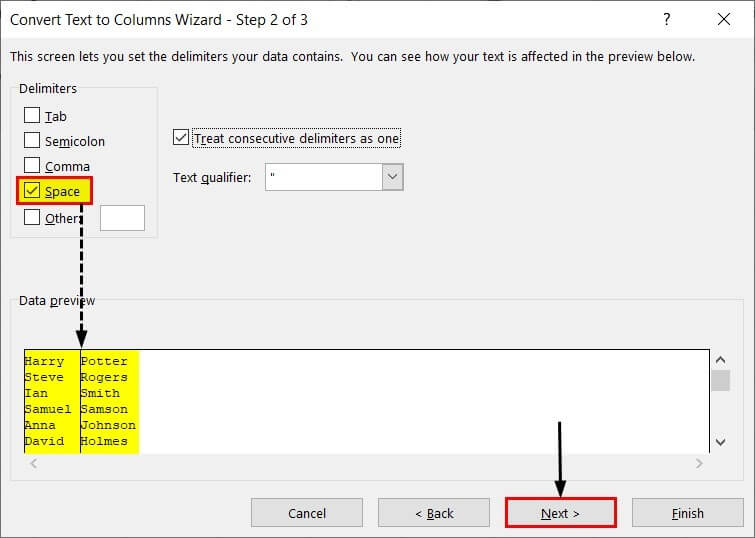
- Under “delimiters,” select the checkbox for space. Deselect the other delimiters (if selected), as shown in the following image. Click “next.”

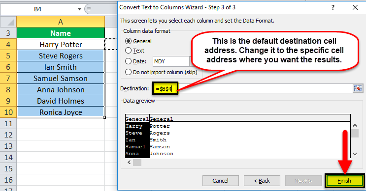
- Under “destination,” specify the cell in which the output is required. Enter “$B$4” and click “finish.”
Note:If you proceed with the default cell address under “destination,” the output will replace the original dataset. To retain the initial data as is, select a cell to its right as the “destination.”

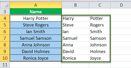
- The output is shown in the following image. The names of column A have been split into the first name (column B) and the last name (column C).
Note:The results of the “text to columns” property are static. This means that any change made to the source data is not reflected in the results. Hence, to include the changes, the whole process has to be repeated.


Example #2–Split by “Fixed Width” Option
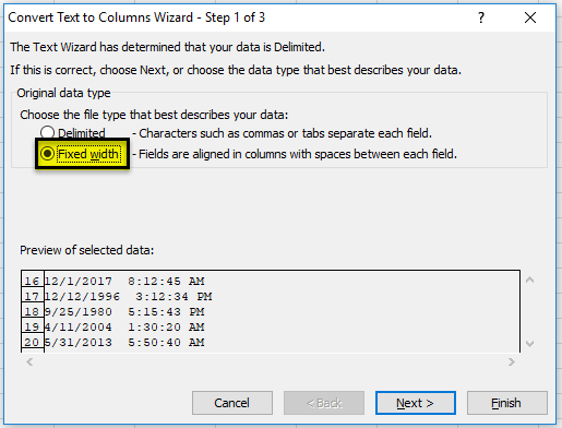
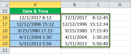
The following list shows the date and time of specific days. We want to split the date and time into separate columns. Use the “fixed width” option of the text to columns wizard.
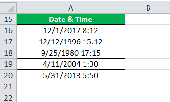
Step 1: Select the range A16:A20, as shown in the following image. In the Data tab, click “text to columns” under the “data tools” group.
Step 2: The “convert text to columns wizard” dialog box appears. Select the option “fixed width,” as shown in the following image. Click “next.”
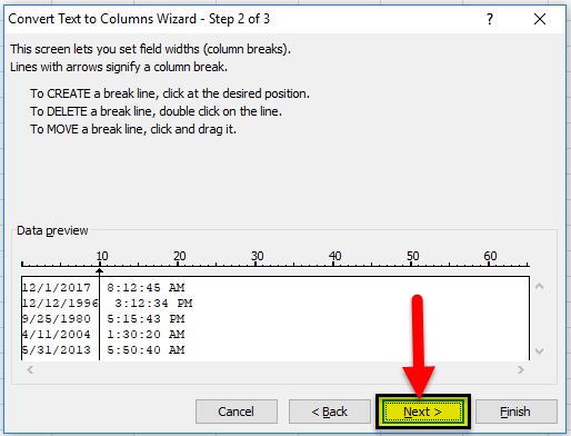
Step 3: Under “data preview,” place a break line (on the text) at the position where splitting is to be carried out.
Since we want to split the date and time, we insert the break line between these two data strings. Click “next.”
Note: To remove the break line, double-click on it.
Step 4: Under “column data format,” select date, as shown in the following image. In “destination,” enter the cell address where the results are required. Click “finish.”
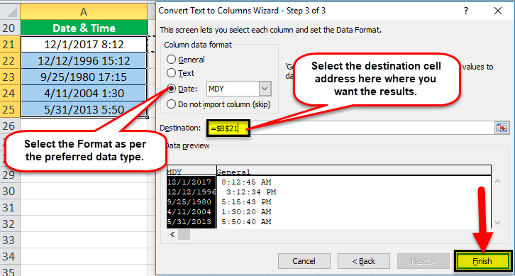
Step 5: The output is shown in the following image. The data strings of column A have been split into the dates (column B) and the time (column C).
Frequently Asked Questions (FAQs)
What is the splitting of cells and how is it done in Excel?
When a cell is split, its components are divided into separate cells. Splitting is often done when there is a need to sort and re-arrange the existing data. Since the substrings of data are moved to new cells, splitting helps to analyze the resulting columns.
To split an excel cell, the text to columns feature is used. This separates the data of a cell, based on either the delimiter character or the fixed length of a substring.
The steps to split cell in excel are listed as follows:
a. Select the cells to be divided. In the Data tab, click “text to columns” under the “data tools” group.
b. Select the option “delimited” or “fixed width.” Click “next.”
c. If “delimited” is selected, enter the required separator in “delimiters.” If “fixed width” is selected, insert the break line at the desired position.
d. Select the “column data format” and specify the “destination.” Click “finish.”
The content of the selected cells is split into different excel columns.
How to split a cell’s content separated by commas into multiple cells of Excel?
Let us split column A which consists of data strings separated by a comma and space.
The entries in the range A1:A5 are listed as follows:
• Jack Adams, Chicago, USA, 2016
• Peter Smith, Houston, USA, 2019
• Ella Taylor, Glasgow, UK, 2018
• Lily Brown, Birmingham, UK, 2015
• Birdie Evans, Paris, France, 2020
The steps to split data into multiple cells using the “delimited” option are stated as follows:
a. In the Data tab, select the option “text to columns.” This is under the “data tools” group.
b. The “convert text to columns wizard” dialog box appears. Select “delimited” under “choose the file type that best describes your data.” Click “next.”
c. Select the checkboxes for both comma and space. Select the checkbox for “treat consecutive delimiters as one.” Click “next.”
d. Select “general” under the “column data format.” Enter “$B$1” under “destination.” Click “finish.”
Five separate columns (columns B to F) are created containing the first names, last names, cities, countries, and years respectively.
Note 1: Before the procedure begins, ensure that there are empty columns to the right of the destination cell. This prevents overwriting the source data.
Note 2: It is recommended to glance through the “data preview” before clicking “finish” in the last step. This ensures that the splitting of data is executed properly.
How to split cells in Excel automatically?
The flash fill feature helps to split cells automatically. When the user enters the split up text in a few cells one by one, Excel senses a pattern and fills the remaining cells.
Let us split the first and the last names of column A containing Jack Adams, Peter Smith, Ella Taylor, Lily Brown, and Birdie Evans (in the range A1:A5).
The steps of splitting excel cells with the help of flash fill are listed as follows:
a. In column B, enter the first name “Jack” in cell B1.
b. Enter “Peter” in the subsequent cell B2.
c. Excel detects a pattern and displays the first names for the remaining cells B3, B4, and B5. Press the “Enter” key.
Column B is filled with the first names (in the range B1:B5).
Note 1: Ensure that the first names in cells B1 and B2 are entered without the double quotation marks.
Note 2: Alternatively, after the first step (step a), click “flash fill” under the “data tools” group of the Data tab. This populates similar data in the remaining cells.
Recommended Articles
This has been a guide to splitting a cell in Excel. Here we discuss how to split a cell in Excel by using the text to columns wizard (delimited and fixed-width method) along with Excel examples and downloadable Excel templates. You may also look at these useful functions of Excel–