Combine Cells In Excel

What Is Combining Excel Cells?

Combine Cells in Excel helps users join the cell values of multiple cells into a single cell to view it as a single value than multiple values.

To Combine Excel Cells, one can use either the ampersand (&) or the CONCATENATE Function of Excel.

For example, we can view the branch location and the number of employees working in a single cell for the Bank Manager to keep track. The formula “=A2&”,”&B2” (exclude the beginning and ending double quotation marks) combines cells A2 and B2 containing “location X” and “570”, respectively.

Therefore, the output is “location X,570.” The comma of this output serves as a separator (delimiter) between the two cell values. This is shown in the following image.

The purpose of Combining Excel Cells is to arrange the data in the desired format. Moreover, it improves the presentation of data, thereby making the dataset suitable for further processing.

It must be noted that Combining Excel Cells is different from merging cells. The latter retains the data of the upper-left-most cell only, while there is no data loss in case of the former.

• Combine Cells in Excel helps users to combine two or more cell valuesto get a new combined values like combining the first name and last name, or entering the location with name details.
• We can Combine Excel Cells using some ways, namely, ampersand (&), Concatenate(), Char(), Text(), and VBA Code.
• The TODAY function we use returns the current date, and updates automatically each time the workbook is opened. It does not take any arguments.
• The TEXT function converts a numeric value to text in the format specified by the user.

How To Combine Cells In Excel?

We can Combine Cells in Excel in the following ways,

1. Combine a Text String and Number with the Ampersand Operator.
2. Combine two Text Strings with the Ampersand and CONCATENATE.
3. Combine two Text Strings and add a Line Break with the Ampersand and CHAR.
4. Prefix and Suffix Text Strings to a Number with the Ampersand.
5. Prefix Text Strings to the Current Date with the Ampersand.
6. Combine Cell Values in VBA with the Ampersand.

Examples

Let us consider specific examples for the above-mentioned methods to understand the process of Combine Cells in Excel.

Example #1 – Combine a Text String and Number with the Ampersand Operator

The image shows the product name and code in columns A and B, respectively.  Let us combine the text string (column A) and the numeric value (column B) of each row in a single cell (in column D).

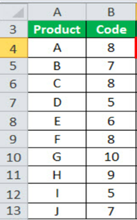
The steps to Combine Cells using the ampersand operator are listed as follows:

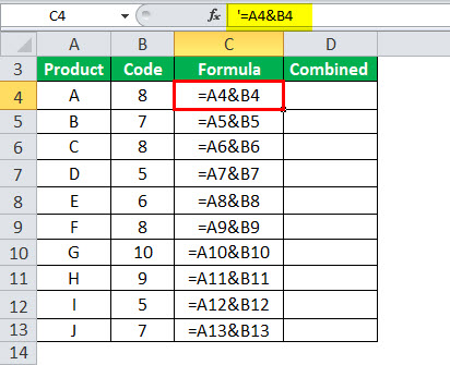
Step 1: Enter the formula “=A4&B4” in cell C4, as shown in the succeeding image.

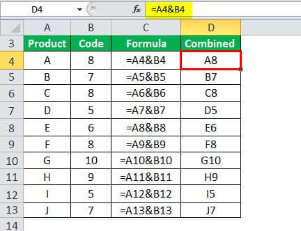
Step 2: Press the “Enter” key. The output for the first row is “A8,” as shown in the succeeding image. To obtain the outputs for all the rows, drag the formula to the remaining cells of the column.

For simplicity, we have retained the formulas in column C and given the outputs in column D. Hence, in the first output, the letter “A” and the number 8 have been combined to form “A8.”

Example #2 – Combine two Text Strings with the Ampersand and CONCATENATE

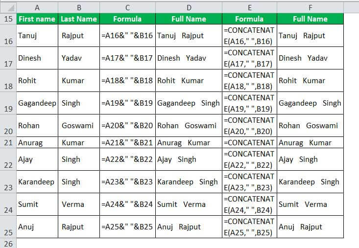
The succeeding image shows the first and last names in columns A and B, respectively. We want to obtain the full names separated by a space within a single column. Use the ampersand operator and the CONCATENATE function to Combine Excel Cells of each row.

The steps to Combine two cell values using the given techniques are listed as follows:

Step 1: Enter the following formulas in cells C16 and E16, respectively.

• “=A16&” “&B16”
• “=CONCATENATE(A16,” “,B16)”

Step 2: Press the “Enter” key after entering each of the preceding formulas. Next, drag the formula to the remaining cells of the column. The outputs are shown in the succeeding image.

For simplicity, we have retained the formulas using the ampersand and the CONCATENATE in columns C and E, respectively. The outputs have been given in columns D and F. Hence, in the first output (D16 and F16), the names “Tanuj” and “Rajput” have been combined to form the full name “Tanuj Rajput.”

, the output also would have had three spaces between the first and the last names .

Example #3 – Combine two Text Strings and add a Line Break with the Ampersand and CHAR

The succeeding image shows the first and the last names in columns F and G, respectively. We want to combine the two names of each row in a single cell (column I). Further, add a line break between the combined names. Use the ampersand operator and the CHAR function.

The steps to combine the names and insert a line break in Excel are listed as follows:

Step 1: Enter the following formula in cell H4, “=F4&CHAR(10)&G4”.

The ampersand combines the first name and the last name. The “CHAR(10)” inserts a line break after the first name and before the last name.

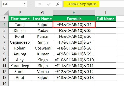
Step 2: Press the “Enter” key. Next, select the output cell, and click "wrap text" from the “alignment” group of the “Home” tab. The final output is shown in cell I4 of the following image.

Hence, in the first output, the names “Tanuj” and “Rajput” have been combined (with a line break in between) to form “Tanuj Rajput.”

To obtain the outputs for the entire column, drag the formula of the preceding step (step 1) to the remaining cells. Next, select the output column and click “wrap text.” For simplicity, we have retained the formulas in Column H and given the outputs to Column I.

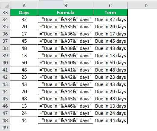
Step 2: Press the “Enter” key. The output is shown in cell C34 of the succeeding image. Drag the formula entered in the preceding step to the remaining range.

For simplicity, we have retained the formulas in column B and given the outputs in column C.

Hence, the given prefix and suffix have been added to all the numeric values of column A. The outputs of column C represent the terms of a payment schedule.

Example #5 – Prefix Text Strings to the Current Date with the Ampersand

We want to prefix the text string “today is” with today’s date. The output should contain the date in the following formats:

• As a serial number of Excel.
• As a text string in the format mm-dd-yyyy.

For both the preceding pointers, use the ampersand operator and the TODAY function. Use the TEXT function as well for the second pointer.

Note that the date of creation of this article was December 1, 2018. So, all the following calculations take into account the given date.

The steps for the given task are listed as follows:

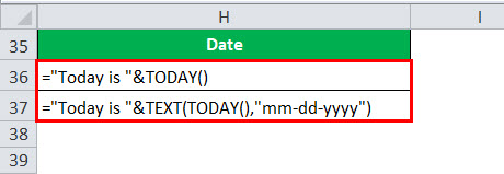
Step 1: Enter the following formulas in cells H36 and H37, respectively.

• “=”Today is “&TODAY()”
• “=”Today is “&TEXT(TODAY(),”mm-dd-yyyy”)”

These formulas are shown in the succeeding image.

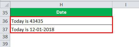
Step 2: Press the “Enter” key after entering the two preceding formulas. The outputs are displayed in the following image.

Hence, in the first output (cell H36), the TODAY function has returned a serial number (43435). This number corresponds to the date of December 1, 2018.

In the second output (cell H37), the date returned by the TODAY function is converted to text (in mm-dd-yyyy format) by the TEXT function. Had we not used the TEXT function, the date would have been displayed as a number.

Therefore, the prefix “today is” has been added to the two date formats with the help of the ampersand operator, as shown below.

Example #6–Combine Cell Values in VBA with the Ampersand

We want to combine the values of cells A4 and B4 in a single Excel cell, C4. Write the VBA code for the same.

The code for Combining the Cell Values (without any data loss) is given as follows:

Sub Mergecells()

  Range(“C4”).Value = Range(“A4”).Value & Range(“B4”).Value

End Sub

Execute the above VBA code in the VBA Editor to get the desired output.

Important Things To Note

• Exclude the beginning and the ending with double quotation marks while entering the preceding formulas in Excel.
• A delimiter is a character or symbol that separates two values.
• While entering the preceding formulas in Excel, ensure that the beginning and ending double quotation marks are excluded.

Frequently Asked Questions (FAQs)

1. Why do we Combine Cells in Excel?

The combining of cells is the joining of the values of two or more cells. We use the CONCATENATE function or the ampersand operator (&) to combine cell values. By combining cells, no data is lost, unlike in the case of merging cells.
We Combine Cells to join similar or related data, to give a continuation of the entered data, to organize data in an order, and for a neat display of the combined output.
It is possible to insert a delimiter, a separator (like space, comma, etc.), or also add a line break, at the relevant places in the combined output.

2. Name some of the delimiters we use to Combine Cells in Excel.

The delimiters required in the combined output should be enclosed within double quotation marks in the formula entered initially.
For example, some of the different delimiters that are available to combine the values of cells A1 and B1 are as follows:
a. Comma: “=CONCATENATE(A1,”,”,B1)” or “=A1&”,”&B1”.
b. Space: “=CONCATENATE(A1,” “,B1)” or “=A1&” “&B1”.
c. Semicolon: “=CONCATENATE(A1,”;”,B1)” or “=A1&”;”&B1”.
d. Hyphen: “=CONCATENATE(A1,”-“,B1)” or “=A1&”-“&B1”.

3. State the Excel formulas (using CONCATENATE and “&”) for combining data in the following cases:
• Three cell values with the space as the delimiter.
• Three cell values with the space as the delimiter and a date (in dddd/mm/yyyy format) in the center of the combined output.

#To combine the values of cells A1, B1, and C1 with spaces in between, use either of the following formulas in Excel:
a. “=CONCATENATE(A1,” “,B1,” “,C1)”
b. “=A1&” “&B1&” “&C1”
#To combine the values of cells A1, B1, and C1 where B1 contains a date (12/01/2021) and the space is the delimiter, use either of the following formulas in Excel:
a. “=CONCATENATE(A1,” “,TEXT(B1,”dddd/mm/yyyy”),” “,C1)”
b. “=A1&” “&TEXT(B1,”dddd/mm/yyyy”)&” “&C1”

Download Template

This article must help understand Combine Cells in Excel with its formulas and examples. You can download the template here to use it instantly.

Recommended Articles

This has been a guide to Combine Cells in Excel. Here we Combine cell values using delimiters, ampersand (&), Concatenate(), examples & downloadable template. You may also look at these useful articles of Excel –

• Combine Text From Two Or More Cells into One Cell
• Concatenate Excel Columns
• Concatenate Strings in Excel
• Count Colored Cells In Excel
• Excel Translate