Table Of Contents
The Techniques of Merge Cells in Excel
The different ways of merging cells in Excel are listed as follows:
- “Merge and center” drop-down
- CONCATENATE function
- Ampersand operator (&)
How to Merge Cells in Excel?
Let us understand how to merge cells in Excel. We discuss the three merging techniques followed by a few more topics. Each topic consists of an example. Thereafter, some relevant examples are taken up.
Method #1 - “Merge and Center” Drop-down
The “merge and center” drop-down consists of various merging options that help combine multiple cells into one. It can be found under the “alignment” group of the Home tab, as shown in the following image.

The different options of the “merge and center” drop-down are explained as follows:
- Merge and center: This merges the selected cells and places the data string in the center. While merging, it retains the text of the upper-leftmost cell only. The text of the remaining merged cells is deleted.
- Merge across: This merges across, implying that the selected cells of the same row are joined together. It merges the values of one row at one time. It retains the text of the upper-leftmost cell only.
- Merge cells: This merges all the selected cells into one single cell. The cells can be selected either horizontally or vertically, or both. It retains the text of the upper-leftmost cell only.
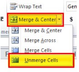
- Unmerge cells: This unmerges the cells implying that the merged cells are split into separate cells again.
Note 1: The difference between the options “merge and center” and “merge cells” is in the alignment of the merged output.
Note 2: The excel shortcut for merging (merge and center) is “Alt+H+M+C” and for unmerging is “Alt+H+M+U.” Both the shortcuts must be pressed one by one.
Example #1
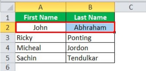
The following table shows the first and the last names in columns A and B respectively. We want to merge the two names with the help of the “merge and center” option.
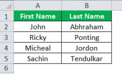
The steps to merge cells with the “merge and center” option are listed as follows:
- Select the cells A2 and B2, which are to be merged.
- From the merge and center drop-down in the Home tab, choose merge and center.
- A message appears stating that only the upper-leftmost data will be retained. Click Ok.

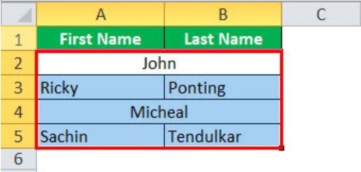
- The cells A2 and B2 are joined with the name John in the center. The output is shown in the following image.
The cells A2 and B2 are merged rather than their values. Hence, the text of cell B2 (Abhraham) is deleted while merging cells.
Method #2 - CONCATENATE Function
The CONCATENATE function combines or concatenates the content of two or more cells. In other words, the values of several cells are joined together in one cell. This function ensures that no data string is lost while merging cell values in excel.
The following image illustrates the CONCATENATE formula for joining the values of cells A2 and B2 with a space in between.
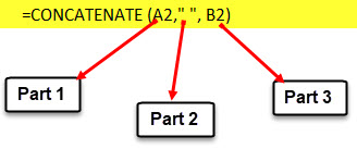
The three parts of the function are explained as follows:
- Part 1 (A2): This is the first cell reference to be joined.
- Part 2 (" "): This is the delimiter “space” that separates the values of the two cells.
- Part 3 (B2): This is the second cell reference to be joined.
Example #2
Working on the data of example #1, we want to merge the first and the last name with a space in between. Use the CONCATENATE function.
The steps to merge cell values with the CONCATENATE formula are listed as follows:
Step 1: Select the cell C2 in which the output is required.
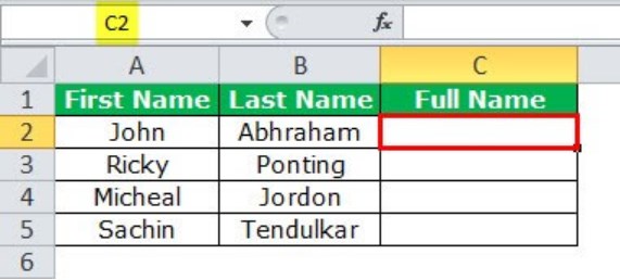
Step 2: Enter the following CONCATENATE formula in cell C2.
“=CONCATENATE(A2," ",B2)”
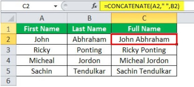
Step 3: Press the “Enter” key. The output appears in cell C2, as shown in the following image.
Hence, the values of cells A2 and B2 are merged.
Method #3 - Ampersand Operator (&)
The ampersand operator combines different text strings by the insertion of “&” within the formula. The formula for combining the values of cells A2 and B2 with a space in between is “=A2&" "&B2”
By using the ampersand, no data string is lost while merging cell values in excel.
Example #3
Working on the data of example #1, we want to join the first and the last name with the help of the ampersand.
The steps to merge cell values with the ampersand operator are listed as follows:
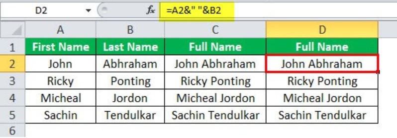
Step 1: Enter the following formula in cell D2.
“=A2&" "&B2”
Step 2: Press the “Enter” key. The output appears in cell D2, as shown in the following image.
Hence, the content of cells A2 and B2 has been merged.
The “Unmerge Cells” Option
Once the cells have been merged, they can be unmerged as well. The “unmerge excel cells” option (under the “merge and center” drop-down) splits the merged cells, thereby returning the initial layout of cells. However, the data values lost in merging are not restored.
Example #4
Working on the data of example #1, we want to unmerge the merged entries in rows 2 and 4. These entries were merged with the “merge and center” option. Use the “unmerge cells” option for unmerging.
The steps to unmerge data are listed as follows:
Step 1: Select the complete data range A2:B5.
Step 2: Click “unmerge cells” from the “merge and center” drop-down under the Home tab.
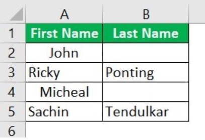
Step 3: The cells in rows 2 and 4 have been unmerged. However, the initial data values of column B (shown in example #1) are not restored.
Note: Alternatively, select the merged entries one by one. Thereafter, apply the “unmerge cells” option separately for each entry.
An Alternate Method for Center Alignment
It is difficult to sort (“sort and filter” group of Data tab) merged cells. This is because sorting a merged range in an ascending or a descending order returns a message stating that the cells need to be “identically sized.”
To overcome this limitation, there is an alternate option which does not merge cells but applies the same formatting as the “merge and center” option. In other words, the cells are aligned centrally without any data strings being lost.
The alternate option “center across selection” is available in the “alignment” tab of the “format cells” dialog box.
Example #5
Working on the data of example #1, we want to apply the same formatting as the “merge and center” option without losing any data. Use the “center across selection” alternative.
The steps to format data with the “center across selection” option are listed as follows:
Step 1: Select cells A2 and B2, which are to be formatted.
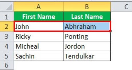
Step 2: Press “Ctrl+1” together. The “format cells” dialog box opens, as shown in the following image.
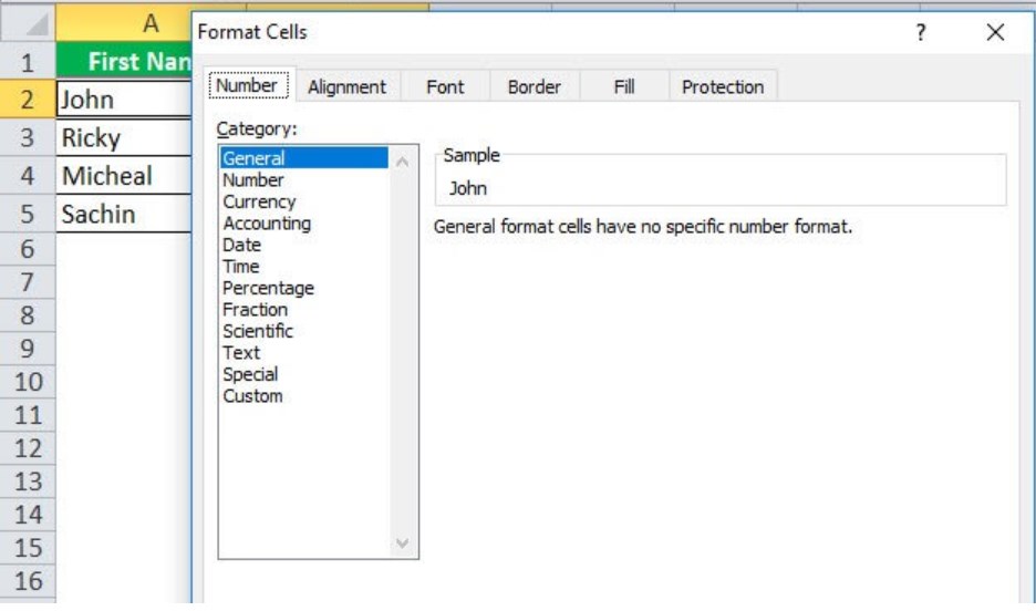
Step 3: Click the “alignment” tab.
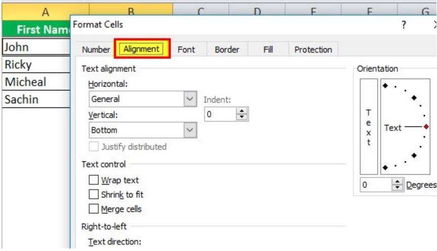
Step 4: Select “center across selection” from the drop-down of “horizontal.” Click “Ok.”
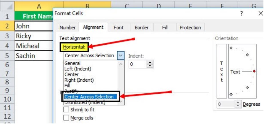
Step 5: The formatted output is shown in row 2 of the following image. Hence, the content of cells A2 and B2 is centrally aligned without any loss of data.
Example #6 - Merge Multiple Cells
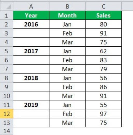
The following table shows the monthly sales (in $) for the years 2016 to 2019. Every year written in column A is followed by two blank cells.
We want to merge the year with the two cells following it so that one cell is created for one year.
The steps to merge multiple cells in Excel are listed as follows:
Step 1: Select the cells A2, A3, and A4.
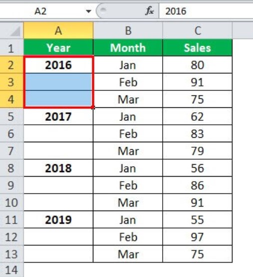
Step 2: Select “merge and center” from the “merge and center” drop-down of the Home tab. In case the message appears, click “Ok” to merge the cells.
Once merged, apply “middle align” from the “alignment” section of the Home tab. Moreover, bold the text “2016.”
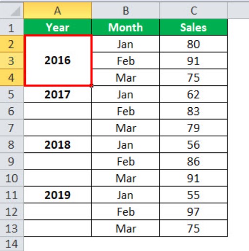
Step 3: Keep the cell containing “2016” selected. Double-click on “format painter" under the Home tab.
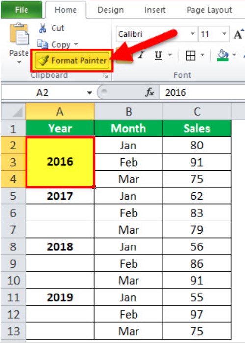
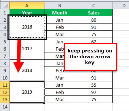
Step 4: For applying the formatting of “2016” to the remaining cells, press the down arrow key. Excel keeps merging the three excel cells for every year till the “escape” key is pressed.
Example #7–Merge the Title Cell
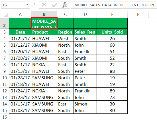
The following table shows the number of units of a particular product sold by the different sales representatives of an organization. In addition, the date of sale (column A) and the respective region (column C) are also displayed.
The cell B2 shows the title of the table, which is not completely visible currently. We want to merge the cells A2:E2 so that the title is spread across columns A to E.
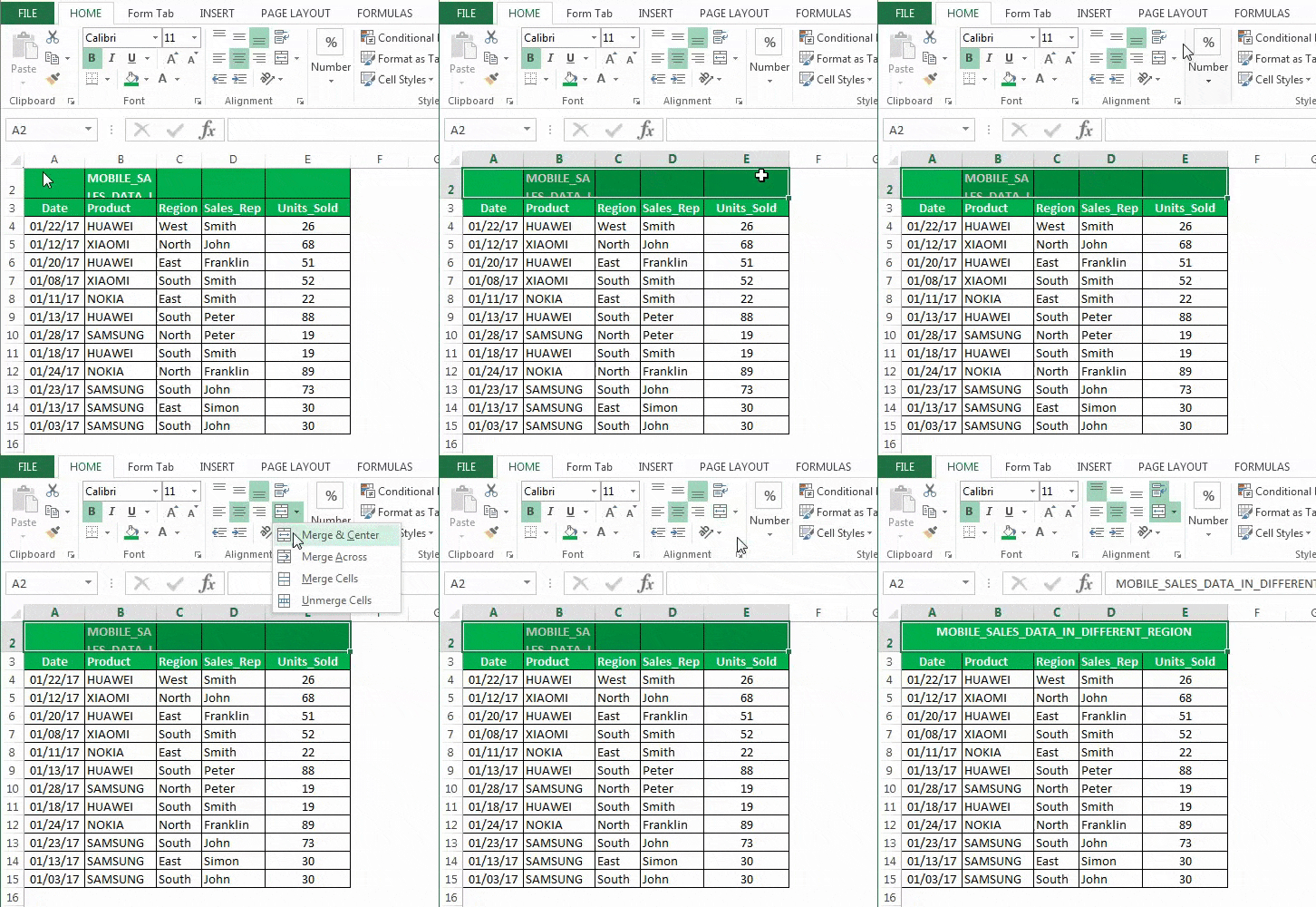
Step 1: Select the cells A2, B2, C2, D2, and E2 to be merged. The selection can be carried out in any of the following ways:
- Select with the mouse.
- Select by pressing and holding “Shift” along with the relevant arrow keys.
The same is shown in the following image.
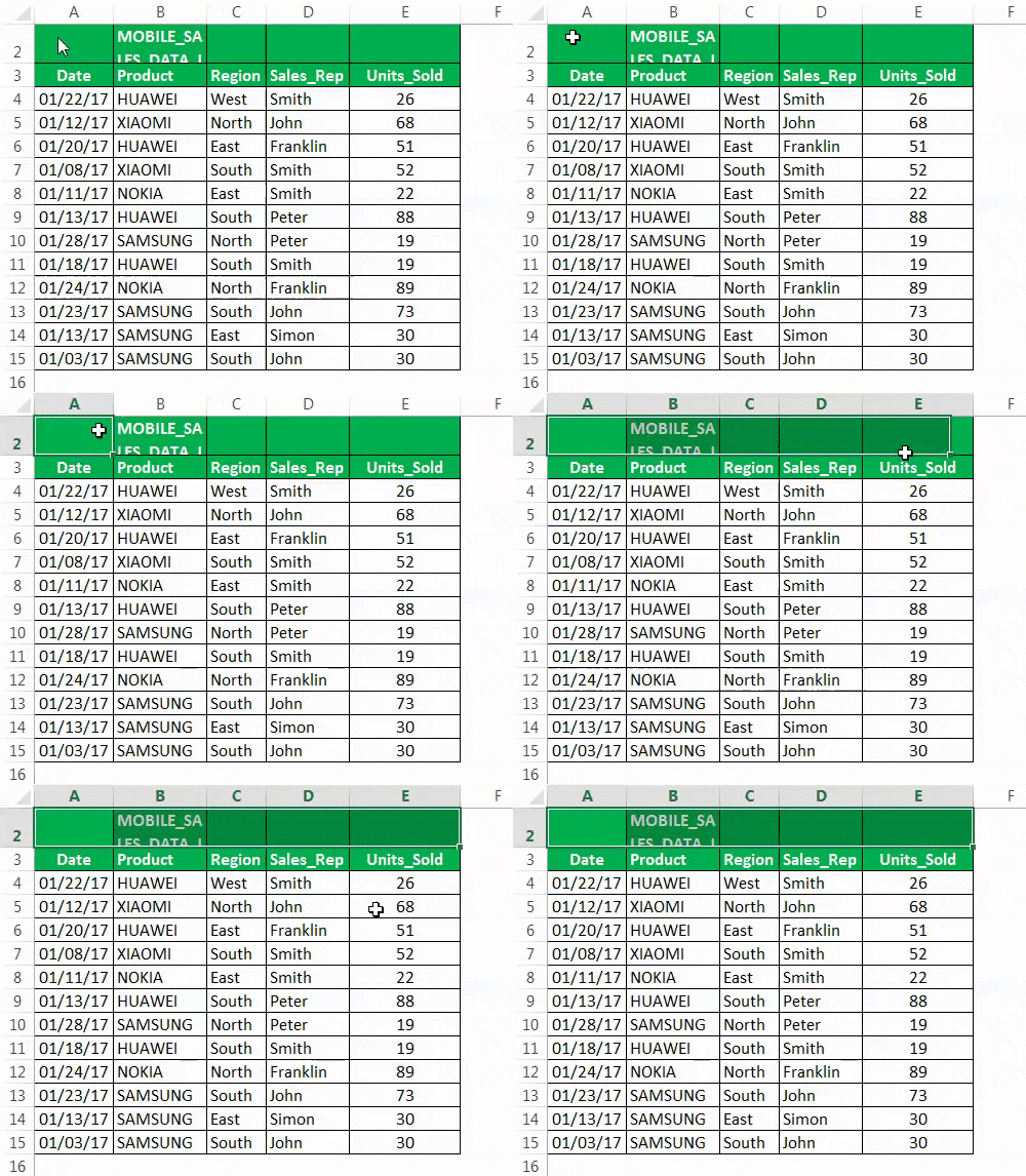
Step 2: Select “merge and center” from the alignment group of the Home tab, as shown in the following image.
Step 3: In this case, Excel will not display the message stating that only the upper-leftmost data will be retained. This is because only cell B2 contains data while the remaining cells (A2, C2, D2, and E2) are empty.
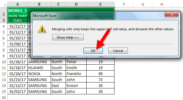
However, if the following message does appear, click “Ok.”
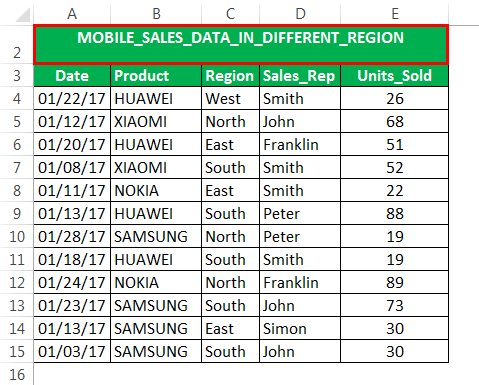
Step 4: The cell range A2:E2 is merged. The title “mobile_sales_data_in_different_region” appears in the center of columns A to E.
To make the title stand out, give it a color.
Example #8–Merge two Column Values With the Ampersand Operator
The following table shows the first and last names in columns A and B respectively. We want to perform the following tasks:
a) Merge the data strings of columns A and B with a space in between.
b) Merge the data strings of columns A and B without any spaces.
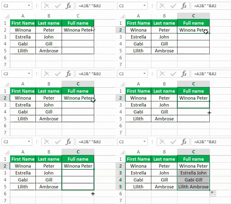
a) Step 1: Select the cell C2 in which the formula for merging data strings is to be entered.
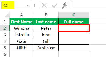
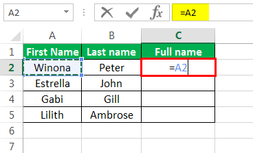
Step 2: In cell C2, enter the operator “equal to” (=) followed by selecting cell A2 (the first cell to be combined).
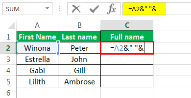
Step 3: Enter the ampersand operator (&) followed by a space enclosed within double quotation marks. Enter another (second) ampersand.
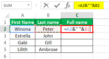
Step 4: Select cell B2, which is the second cell to be combined. After entering the complete formula (=A2&" "&B2), press the “Enter” key.
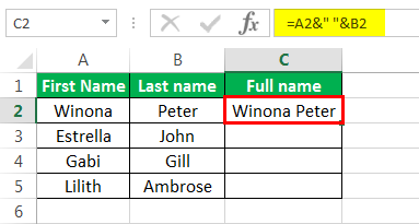
Step 5: The merged output appears in cell C2. Hence, the first and the last names have been combined with a space in between.
Step 6: Drag the formula to the remaining cells. Hence, the full names (with a space in between) for the entire range (C2:C5) are obtained.
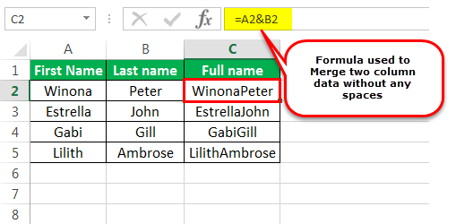
b) We apply the following formula in cell C2.
“=A2&B2”
Press the “Enter” key. Drag the formula to obtain the output in the remaining cells.
The formula merges the values of columns A and B without any spaces between the data strings. The merged output is shown in the following image.
Example #9–Merge two Column Values With the Concatenate Function
Working on the data of example #8, we want to merge the first and the last name with a space between them. Use the CONCATENATE function of Excel.
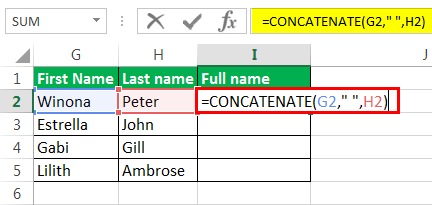
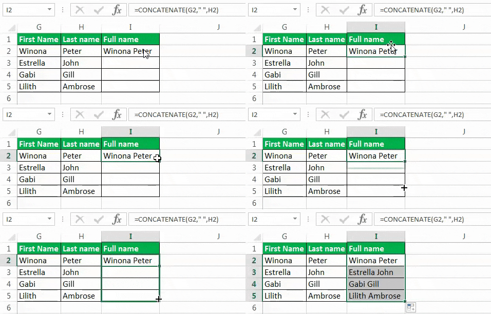
Step 1: Enter the following formula in cell I2.
“=CONCATENATE(G2," ",H2)”
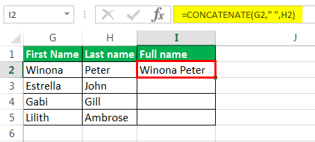
Step 2: Press the “Enter” key. The merged output is shown in the following image.
Hence, the names of cells G2 and H2 are joined with a space in between.
Step 3: Drag the formula to obtain the output in the remaining cells. Hence, the full names (with a space in between) for the entire range (I2:I5) are obtained.
The Limitations of Merging Excel Cells
The drawbacks of merging cells in Excel are stated as follows:
- While merging with the “merge and center” drop-down, only the upper-leftmost data is retained and the remaining data is deleted.
- The merging options of the “merge and center” drop-down merge only the excel cells, not their values.
- Once merged, it becomes difficult to sort data whether in an ascending or a descending order.
Note: It is recommended to use the merging options of the “merge and center” drop-down in worksheets that are just meant for presentation purposes. In addition, limit the usage of these options to headings and cell titles only.

