New Line in an Excel Cell

Last Updated :

21 Aug, 2024

Blog Author :

Edited by :

Reviewed by :

Table Of Contents

Insert a New Line in an Excel Cell

A new line in excel cell is inserted when one needs to move a string to the next line of the cell. To insert a new line, a line break must be added at the relevant place. A line break tells Excel to break the existing line and begin a new line (within the same cell) with the immediately following character. When line breaks are inserted in a cell, its content can be seen in multiple lines.

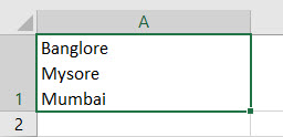
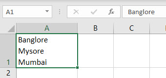
For example, in the following image, a line break has been inserted after the cities Bangalore and Mysore. So, a total of two line breaks have been inserted in cell A1. Notice that the three cities are in three different rows of the same cell.

Starting a new line in an excel cell ensures that the lengthy text strings are split into multiple lines. This improves the readability and lends a neat look to the worksheet. To obtain the right result after inserting line breaks, ensure that the wrap text feature of Excel is turned on.

Insert a New Line in an Excel Cell

Top 3 Ways to Insert a New Line in a Cell of Excel

The methods to start a new line in a cell of Excel are listed as follows:

Shortcut keys “Alt+Enter”
“CHAR(10)” formula of Excel
Named formula

Let us consider an example of each technique.

Note: The line feed (LF) and carriage return (CR) are two terms closely related to a line break. The LF moves the cursor to the next line within the cell. In contrast, a CR moves the cursor to the beginning (or the first position) of the same line. So, with a CR alone, the cursor does not move to the next line.

Every operating system considers a line break (LF or CR or a combination of CR and LF) differently. For instance, when a line break is inserted in the Windows operating system, both CR and LF (called CR+LF or CRLF) are inserted together.

The CRLF moves the cursor to the beginning of the next line. However, the “Alt+Enter” method inserts only line feeds in Excel. The ASCII (American Standard Code for Information Interchange) codes for LF and CR are 10 and 13 respectively.

In this article, the usage of code 10 has been shown in example #2. Further, this article uses the term line break in place of line feed and carriage return. Hence, consider all three (line break, line feed, and carriage return) to be the same in this article.

#1 – Using the Shortcut Keys “Alt+Enter”

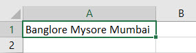
The following image shows the names of three cities of India in cell A1. We want to insert a line break after the first two cities of this cell. Use the keys “Alt+Enter” of Excel.

The steps to insert line breaks by using the keys “Alt+Enter” are listed as follows:

Step 1: Double-click inside cell A1. Next, move and bring the cursor immediately before the “M” of Mysore. To do this, either move the cursor with the arrow keys of the keyboard or click at the stated position with the left-click of the mouse.

The cursor is placed before Mysore because a line break needs to be inserted at this position.

Note: Alternatively, one can also place the cursor at the stated position in the formula bar.

Step 2: Press the keys “Alt+Enter.” For this shortcut to work, hold the “Alt” key while pressing the “Enter” key.

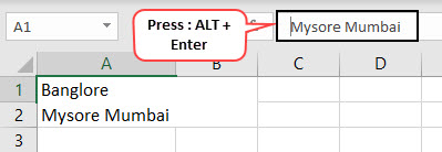
A new line is inserted before “Mysore,” as shown in the following image.

Step 3: Place the cursor before the “M” of Mumbai by using the left-click of the mouse. Press the keys “Alt+Enter,” the way they were pressed in the preceding step.

The name “Mumbai” shifts to a new line within the same cell of Excel. This is shown in the following image.

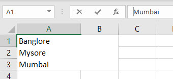
Step 4: Press the “Enter” key to exit the Edit mode. The following image shows the names of the three cities in multiple lines of a single cell (cell A1) of Excel. This result will be displayed only if the wrap text feature of Excel is turned on.

Notice that the formula bar (in the following image) shows a line break after Bangalore.

Note: The “wrap text” is a toggle button in the “alignment” group of the Home tab. It can also be accessed from the “alignment” tab of the “format cells” window. This window can be opened by pressing the shortcut “Ctrl+1.”

By default, the wrap text feature is turned on when a line break is inserted with the “Alt+Enter” method in Excel. To cross-check, keep cell A1 selected and notice that the “wrap text” button is automatically activated after inserting a line break with the shortcut keys.

If the wrap text button is turned off, the content of cell A1 will display in a single line. However, the line breaks will still be visible in the formula bar.

#2–Using the “CHAR(10)” Formula of Excel

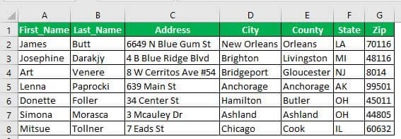
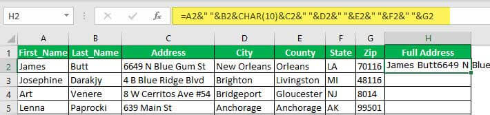
The following image shows the names and addresses of some people. The first and the last names have been split into columns A and B respectively. The address has been split into columns C to G. We want to perform the following tasks:

Join the first and the last name to the full address of each person. For this, combine the strings of columns A and B with those of columns C to G. Use the ampersand (&) to join the stated strings. Ensure that a single space character precedes each string of the address.
Insert a line break between the last name and the first character of the address. Use the CHAR function for inserting line breaks.

In the end, the complete name should be in one line, followed by the address in the subsequent lines of the cell. Further, use a single formula for performing the given tasks. Explain the formula used.

The steps to perform the given tasks by using the ampersand and the CHAR function are listed as follows:

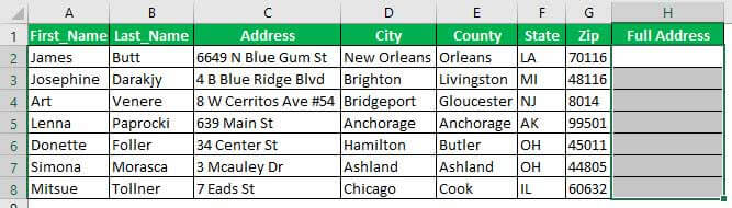
Step 1: Insert a new column to the right of the given dataset. We have inserted column H titled “full address.” This is shown in the following image.

Step 2: Begin by combining the first and last names (of row 2) with the ampersand. To do this, type the following formula in cell H2.

“=A2&“ ”&B2&”

This formula joins the first and the last names of cells A2 and B2 and also inserts a space between them. However, the formula is currently incomplete.

Step 3: Extend the preceding formula to include the CHAR function. Open this function by typing “CHAR,” followed by the opening parenthesis.

The opening of the CHAR function is shown in the following image.

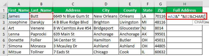
Step 4: Insert the number 10 within the CHAR function. The “CHAR(10)” formula inserts a line break in Excel.

Note: The syntax of the CHAR function is “CHAR(number).” This function returns a character when a number between 1 and 255 is entered. The character is returned from the character set of the user’s computer.

Earlier, the Windows operating system used the ASCII and the ANSI character sets, which have now been replaced by Unicode. The ASCII stands for American Standard Code for Information Interchange. The ANSI character set was created by the American National Standard Institute.

In contrast, the Macintosh operating system uses the Macintosh character set. So, the Macintosh users may use the formula “CHAR(13)” to insert a line break in Excel.

Step 5: Insert the cell references to be joined with the strings of cells A2 and B2. So, in cell H2, enter the following formula by excluding the beginning and ending double quotation marks.

“=A2&" "&B2&CHAR(10)&C2&" "&D2&" "&E2&" "&F2&" "&G2”

Press the “Enter” key. The output appears in cell H2. The formula and the output are shown in the following image. The output is not fully visible as it is in a single line of cell H2 of Excel.

Explanation of the formula: The preceding formula joins the first and the last names (in cells A2 and B2) with the entire address of a person (in cells D2, E2, F2, and G2). The ampersand (&) is used to join.

Notice that, in the formula, a space character has been inserted preceding the strings of cells D2, E2, F2, and G2. This space character is inserted within double quotation marks (like “ ”). These spaces of the formula ensure that spaces are inserted as separators in the output. Moreover, the separators are inserted at exactly those places (in the output) where they have been entered in the formula.

However, no space is inserted between the strings of cells B2 and C2. Rather, the “CHAR(10)” has been used in place of a space. This is because the “CHAR(10)” moves the immediately following string (of cell C2) to the next line.

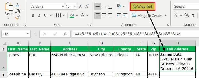
Step 6: Activate the wrap text feature of Excel to see the entire content of cell H2. So, select cell H2 and click the “wrap text” button in the “alignment” group of the Home tab.

The output is shown in the following image. The full name and the complete address are visible in cell H2. Not only the strings of cells A2 to G2 have been joined, but a line break has also been inserted after the name (James Butt). As a result, a legible output has been obtained in cell H2.

Note: When a line break is inserted by the CHAR function, the wrap text feature of Excel is not turned on by default. Rather, this feature needs to be enabled manually to see the impact of the line break.

Step 7: Drag the formula of cell H2 till cell H8 by using the fill handle. The fill handle is displayed at the bottom-right corner of cell H2.

The dragging of the fill handle and the outputs are shown in the following image. Hence, the names and addresses have been consolidated neatly in column H.

#3–Using the Named Formula

Working on the dataset of example #2, we want to perform the following tasks:

Assign the name “NL” to the “CHAR(10)” formula. By doing this, “CHAR(10)” becomes a named formula.
Add the comment “new line inserter” to the name “NL.”
Show how to use the name “NL” (representing the named formula) in the ampersand and CHAR formula of example #2. Explain the formula thus used.

Use the “define name” property of Excel for the first two bullet points.

The steps to perform the given tasks by using the named formula are listed as follows:

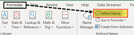
Step 1: Click “define name” from the “defined names” group of the Formulas tab. This option is shown in the following image.

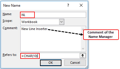
Step 2: The “new name” window opens, as shown in the following image. Make the following insertions in this window:

In the “name” box, enter the name “NL.”
In the “scope” box, let the option “workbook” remain selected.
In the “comment” box, enter the string “new line inserter.”
In the “refers to” box, enter the formula “=CHAR(10).”

Ensure that the insertions of points “a,” “c,” and “d” are entered without the beginning and ending double quotation marks. Click “Ok” once the insertions are done.

Note 1: The name and the comment cannot exceed 255 characters in length. The name must begin with a letter, underscore (_) or backslash (). Further, the name should not consist of any space characters.

Note 2: The “new name” window can also be opened by clicking “name manager” (in the “defined names” group) from the Formulas tab and then clicking “new” (in the “name manager” window).

Step 3: Use “NL” in place of “CHAR(10)” in the following formula.

“=A2&" "&B2&NL&C2&" "&D2&" "&E2&" "&F2&" "&G2”

Press the “Enter” key. The outputs are shown in the following image.

Note: When the “N” of “NL” is typed in the formula, Excel shows the name (NL) as well as the comment (new line inserter) in a list of suggestions. To select “NL” from this list, just double-click it.

Explanation of the formula: The outputs of the preceding formula are the same as that of example #2 (in step 7). This is because other than the name “NL,” the formulas of the two examples (examples #2 and #3) are the same.

Since “CHAR(10)” has been named “NL,” we have used this name in the formula instead of the CHAR function. The “wrap text” feature has also been applied to cell H2. This is the reason its content has fitted into multiple lines of cell H2 of Excel.

Notice that using a different name for “CHAR(10)” has not impacted the result. Rather, using the name “NL” has made the preceding formula compact and understandable.

Note: In this example, “CHAR(10)” is considered a named formula. A named formula is one that has been assigned a name in Excel. Assigning a name (like “NL”) to a formula helps refer to the formula by its name.

So, every time one needs to use “CHAR(10)” in the formulas of the current workbook, one can use “NL” in its place. This is because the “scope” in the “new name” window has been set as “workbook.”

Frequently Asked Questions

1. What does it mean to insert a new line in a cell of Excel? Suggest the shortcuts for inserting a line break in Windows and Macintosh operating systems.

Inserting a new line means moving the content of a cell to the next line. This allows one to break lengthy text strings and display their data in multiple lines of a single cell. The shortcuts for inserting a line break in Excel are stated as follows:

Windows operating system – The shortcut is “Alt+Enter.” For this shortcut to work, hold the “Alt” key while pressing the “Enter” key.

Macintosh operating system – The shortcut is “Control+Option+Return” (or “Control+Command+Return”). For this shortcut to work, hold the “Control” and the “Option” keys while pressing the “Return” key.

Note: Before using the preceding shortcuts, ensure that the cursor is placed where a line break needs to be inserted.

2. How to use the CONCATENATE function and the Find and Replace feature to insert a new line in Excel?

The CONCATENATE function joins the values of different cells in a single cell. Thereafter, the “CHAR(10)” inserts line breaks in the single output cell.

The CONCATENATE and CHAR formula for inserting a new line in Excel is stated as follows:
“CONCATENATE(cell1,CHAR(10),cell2,CHAR(10),cell3,CHAR(10)…)”

The steps for inserting a new line with the Find and Replace feature of Excel are listed as follows:

a. Select the cells in which a new line needs to be inserted.
b. Press the keys “Ctrl+H” to open the Replace tab of the Find and Replace window. Alternatively, click the “find & select” drop-down from the “editing” group of the Home tab. Then, select the “replace” option.
c. In the “find what” box, type the separator that separates the strings. For instance, if a comma separates the strings, type a comma. Likewise, if a space separates the strings, type a space.
d. In the “replace with” box, press the keys “Ctrl+J.” A small, blinking dot appears in this box.
e. Click “replace all.”

In the selected cells, all occurrences of the separator (typed in step “c”) will be replaced by line breaks.

Note: Use the Find and Replace feature for inserting line breaks when each selected cell contains at least one occurrence of the separator. At the same time, there is a need to replace all these occurrences with line breaks.

3. How to remove a line break from a cell of Excel?

The formula to remove a line break from a cell is stated as follows:
“=SUBSTITUTE(cell1,CHAR(10),"")”

The formula to insert a comma in place of a line break is stated as follows:
“=SUBSTITUTE(cell1,CHAR(10),",")”

In both the preceding formulas, “cell1” is the cell that contains the string with line breaks. Further, the SUBSTITUTE function replaces every occurrence of “CHAR(10)” with a blank (“”) or a comma (“,”).

Note: Alternatively, the line breaks can be removed with the Find and Replace feature. Press the keys “Ctrl+J” in the “find what” box. In the “replace with” box, type a separator (like a space or comma) that needs to be inserted in place of a line break. Click “replace all” at the end.

Since removing line breaks with the Find and Replace feature may not always work as desired, one can use the preceding SUBSTITUTE and CHAR formulas.