Formatting Text In Excel

Formatting text in Excel includes color, font name, font size, alignment, font appearance in bold, underline, italic, background color of the font cell, etc.

With formatting, we can add personalized presentation that meets our requirements and expectations.

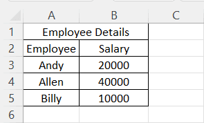
For example, consider the below data.

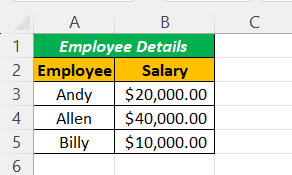
With formatting, we can convert the data as shown in the below image.

Likewise, we can format text in Excel.

In this article, let us learn how to format text in Excel.

• Formatting text in Excel includes font color, size and style, alignment, and cell background color.
• Efficient text formatting in Excel can save time and effort. Learn and use shortcut keys to increase productivity and streamline workflow. Invest time in mastering these shortcuts for higher efficiency in Excel operations.
• Conditional formatting is a feature that allows us to apply specific formatting to text values based on certain conditions. This can be very useful to highlight important data or to identify trends in a table of data.

#1 - Text Name

We can format the text font from default to any other available fonts in Excel. Likewise, we can insert any text value in any of the cells.

Under the "Home" tab, we can see so many formatting options available.

Formatting has been categorized into six groups: "Clipboard," "Font," "Alignment," "Number," and "Styles."

In this, we are formatting the font of cell value A1, "Hello Excel." For this, under the "Font" category, click on the "Font Name" drop-down list and select the font name as per wish.

We hover over one of the font names above. We can see the quick preview in cell A1. If you are satisfied with the font style, click on the name to fix the font name for the selected cell value.

#2 - Font Size

Similarly, we can also format the font size of the text in a cell. Just type the font size in numbers next to the font name option.

Enter the font size in numbers to see the impact.

#3 - Text Appearance

We can modify the default view of the text value. For example, we can make the text value look bold, italic, and underlined. Look at font size and name options. We can see all these three options.

As per the format, we can apply formatting to text value.

• We have applied the "Bold" formatting using the Ctrl + B shortcut excel key.

• To apply "Italic" formatting, use the Ctrl + I shortcut key.

• To apply "Underline" formatting, use the Ctrl + U shortcut key.

• The below image shows a combination of all the above three options.

• If we want to apply a double underline, click on the drop-down list of underline options and choose "Double Underline."

#4 - Text Color

We can format the default font color (black) of text to any colors available.

• Click on the drop-down list of the "Font Color" option and change as per choice.

#5 - Text Alignment

We can format the alignment of the Excel text under the "Alignment" group.

• We can do a left alignment, right alignment, middle alignment, top alignment, and bottom alignment.

#6 - Text Orientation

The important thing under "Alignment" is the "Orientation" of the text value.

Under "Orientation," we can rotate text values diagonally or vertically.

• Angle Counterclockwise

• Angle Clockwise

• Vertical Text

• Rotate Text Up

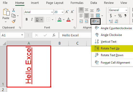
• Rotate Text Down

• Under "Format Cell Alignment, we have many options. Click on this option and experiment with some techniques to see the impact.

Let us see how to apply conditional formatting to text in Excel.

We have learned some of the basic text formatting techniques. How about the idea of formatting only a specific set of values from the group? If we want to find only duplicate values or find unique values.

These are possible through the conditional formatting technique.

For example, look at the below list of cities.

From this list, let us learn some formatting techniques.

#1 - Highlight Specific Value

If we want to highlight only the specific city name, we can only highlight specific city names. For example, assume we want to highlight the city "Bangalore," then select the data and go to conditional formatting.

Click on the drop-down list in excel of "Conditional Formatting" >>> "Highlight cells Rules" >>> "Text that Contains."

Now, we will see the below window.

Next, we must enter the text value that we need to highlight.

Now from the drop-down list, we must choose the formatting style.

Click on "OK." Consequently, it will highlight only the supplied text value.

#2 - Highlight Duplicate Value

To highlight duplicate values in excel, follow the below path. "Conditional Formatting" >>> "Highlight cells Rules" >>> "Duplicate Values."

Again from the below window, we must select the formatting style.

As a result, it will highlight only the text values that appear more than once.

#3 - Highlight Unique Value

Like how we have highlighted duplicate values similarly, we can highlight all the unique values, i.e., text value that appears only once. Then, the formatting window chooses the "Unique" value option from the duplicate values.

It will highlight only the unique values.

• We must learn shortcut keys to format text values in Excel quickly.
• We can use conditional formatting to format some text values based on certain conditions.

This article is a guide to formatting text in Excel. We discuss formatting text using text name, font size, appearance, color, etc., with practical examples and downloadable Excel templates. You may learn more about Excel from the following articles: -

• Conditional Formatting in Dates
• Conditional Formatting along with Formulas
• Combine Text From Two Or More Cells