Scroll Bars in Excel

There are two scroll bars in Excel: a vertical scroll bar is used to view the data in Excel from up and down, and another scroll bar is a horizontal scroll bar used to view the data from left to the right. We can hide or unhide the scroll bar from the "Options" category in the "Files" tab, where we will find the "Advanced" tab and the option to hide scroll bars.

Scroll Bars in Excel

If you have a huge set of data inserted into the Microsoft Excel spreadsheet, you will surely need to use the function of scrollbars in Excel. The interactive scrollbar in Microsoft Excel is very beneficial for users to use Excel when filled with lots of data. You do not have to type a particular value manually to go to the required cell. You can easily use the scroll bar to select the values from a supplied list, saving your time. Let us show you how to create a scroll bar in Microsoft Excel.

Table of contents

• Scroll Bars in Excel
  • How to Create a Scroll Bars in Excel?
  • Resetting the Scroll Bars in Excel – Tiny Scrollbar Error
  • Things to Remember
  • Recommended Articles

How to Create Scroll Bars in Excel?

Let us can understand the process of creating scroll bars in Excel with examples. However, once you are done going through the examples, you might want to check some more instances of the usage of Excel functions. You can check Crash Course In Excel LOOKUP Function for the same.

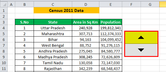
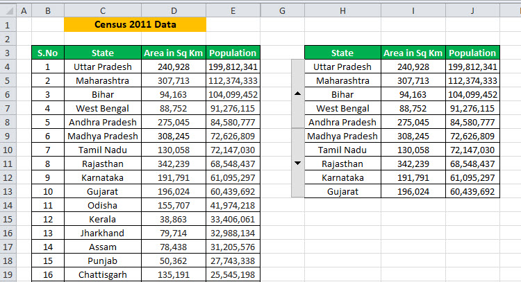
We have taken the data of 35 states in India, according to the census 2011. You can see in the screenshot below that the data is not viewable in the full format on a single screen.

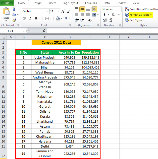
Now, we will create scroll bars in Excel for the above data set, with the help of which a window will display only 10 states at a time. When you change the scroll bar, the data will change dynamically. For better understanding, let us follow the procedures, which have been explained with screenshots.

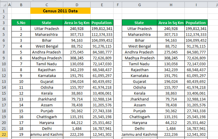
• You have to get your data in place in a managed way. You can see it in the screenshot given below.

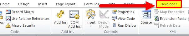
• You must activate the Excel "Develope" Tab in your Excel spreadsheet in case it is not yet started.
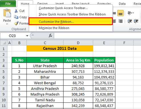
• To activate the "Developer" tab, right-click on any existing Excel tabs and select Customize the Ribbon in Excel.

• You will see the "Excel Options" dialog box. Next, you must check the "Developer" option under the "Main" tab-pane on the right-hand side. Consider the screenshot below.

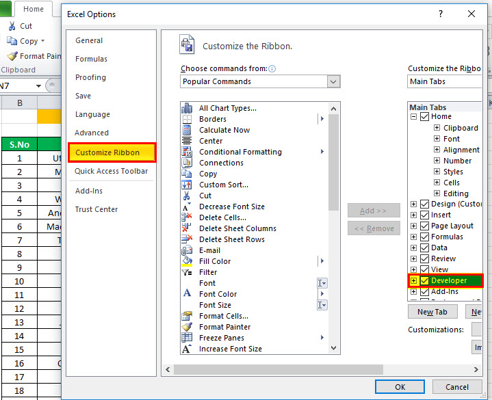
• Now, you will have "Developer" as a tab option.

• Go to the "Developer" tab and click "Insert." Then, under the "Form Control" section, you have to select the "Spin Button (Form Control)."

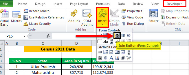
• You have to click the scroll bar in the Excel option and then click any cell of your Excel spreadsheet. You will see the scrollbar inserted in the spreadsheet.

You must right-click on the inserted scroll bar in Excel and select "Format Control." You will see a "Format Control" dialog box.

• Move on to the "Control" tab of the "Format Control" dialog box and make the below-given changes:
• Current Value – 1
• Minimum Value – 1
• Maximum Value – 19
• Incremental Change – 1
• Cell Link – $L$3

See the screenshot below.

• Resize the scroll bar in Excel and place it to fit the length of 10 columns. See the screenshot below.

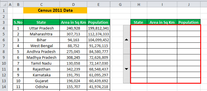
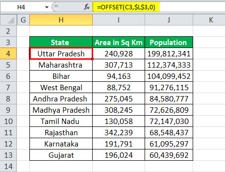
• Now, you have to enter the following OFFSET formula in the first cell of the data, i.e., H4. The formula is =OFFSET(C3,$L$3,0). You have to copy this formula to fill all the other cells of the column.

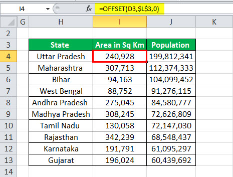
• Similarly, you must insert the OFFSET formula in the I and J columns. The formula for the I column will be =OFFSET(D3,$L$3,0) to be put on cell I4 and for the J column.

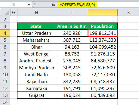
• It will be =OFFSET(E3,$L$3,0) in column J4. Copy the formula to the other cells of the column.

• The above OFFSET formula is now dependent on cell L3 and linked to Excel's scroll bars. The scrollbar is all set for you in the Excel spreadsheet. See the screenshot below.

Resetting the Scroll Bars in Excel – Tiny Scrollbar Error

Sometimes, an issue might arise from the tiny scrollbar. For example, it is very well known that the used range cell size sets both scroll bars, horizontal or vertical. Often, the used range becomes very large due to lots of data sets. Therefore,  the scrollbar may become tiny. This tiny scrollbar issue is so weird that it can make it more difficult for you to navigate around the worksheet.

Let us know why this error happens? It is always caused due to user error only. It can occur if you accidentally stray into the cells way outside of the area, which is needed. This potential human error is responsible for this error to be happening. There are four ways by which you can fix this problem:

1. First, use the "Esc" option and "Undo."
2. Second, delete the cells and save.
3. Third, delete the cells and run the macro.
4. Finally, do it all with a macro.

Things to Remember

• The scrollbar function is useful for Microsoft Excel users when viewing many datasets in a single window.
• We can easily use the scroll bars in Excel for selecting the values from a supplied list, which also saves your time.
• We must activate the "Developer" tab if it is not yet started.
• An error known as "tiny scrollbar" occurs due to human error.

Recommended Articles

This article has been a step-by-step guide to scroll bars in Excel. Here, we discuss its uses and how to create scroll bars in Excel, along with Excel examples and downloadable Excel templates. You may also look at these useful functions in Excel: -

• Scenario Manager in Excel
• Checkbox in Excel
• Combo Box Excel
• Excel Tables