Highlight Every Other Row In Excel

Last Updated :

Blog Author :

Edited by :

Reviewed by :

Table Of Contents

How To Highlight Every Other Row In Excel?

We can make the data we are working on presentable or eye-catching using many features provided by Excel. A few features include changing Font/Text Style, Colour, Size, etc. We can also provide special effects like shading or Highlighting Every Other Row In Excel.

We can highlight every other row in Excel in the following ways, namely:

Using Excel Table
Using Conditional Formatting
Using Custom Format.

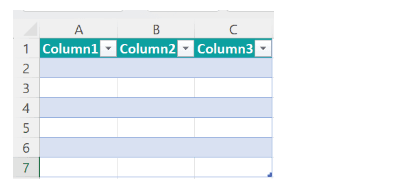
For example, select a cell range, A1:A7, and press “Ctrl+T” shortcut to “Create Table”.

We get a table that automatically Highlights Every Other Row In Excel, as shown above.

How To Highlight Every Other Row In Excel?

Highlight Every Other Row In Excel is a featurethat helps us highlight or give a specific color coding for a specific condition or criteria in a dataset.
We can change the data table to an Excel table to automatically highlight alternate rows and columns, use conditional formatting to create a new rule with a formula to highlight the rows/columns that fulfill a specific condition, or customize as per our requirement.
This feature makes the data more presentable, and the important points stand out.

Download Template

This article must help understand Highlight Every Other Row In Excel with its features and examples. You can download the template here to use it instantly.

Examples

We will consider specific examples for the above-mentioned ways to Highlight Every Other Row In Excel.

Example #1 - Highlight Rows Using Excel Table

In Excel, by default, we have a tool called “Excel Table”.

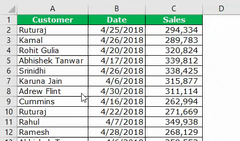
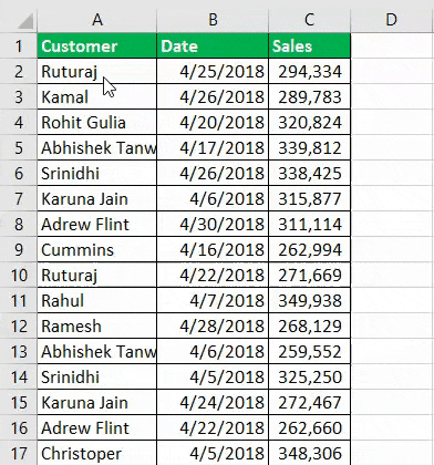
Now, take a look at the raw data.

The steps for highlighting rows using an Excel table are as follows:

First, we must select the data.
Press "Ctrl + T" (shortcut to create table). It will open up the below box.
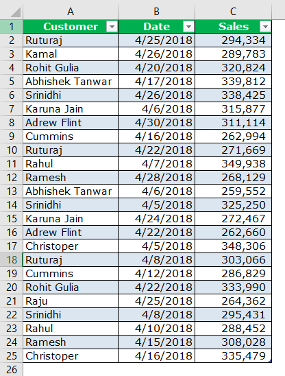
Click on the "OK." It will create a table like this.

It will automatically highlight every other row.
Go to "Design" → "Table Styles."

Here, we have many different types of highlighting every other row by default.

Example #2 - Highlight Rows Using Conditional Formatting

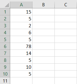
We have a number list from A1 to A10. We want to Highlight Rows Using Conditional Formatting.

The steps tohighlight the number 5 in this range with yellow color are as follows:

Step 1: Select the data range from A1 to A10.

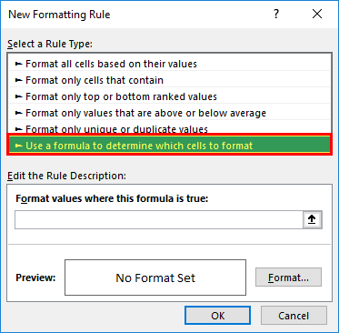
Step 2: Go to the “Home” tab → “Conditional Formatting” → “New Rule.”

Step 3: Now, click on “New Rule.” It will open a separate dialog box. Select “Use a formula to determine which cell to format.”

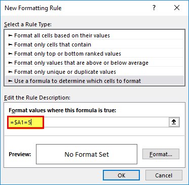
Step 4: In the formula section, we must mention = $A1 = 5.

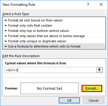
Step 5: Once the formula is inserted, click “Format.”

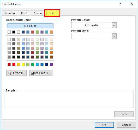
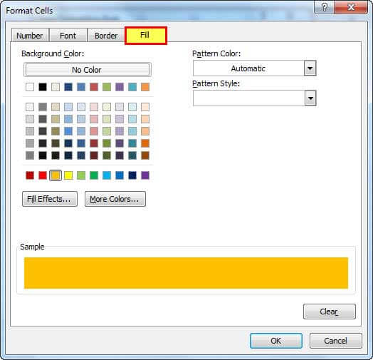
Step 6: Go to the “Fill” option and select the color as per your wish.

Step 7: Click “OK.” As a result, now, it will highlight all the cells containing the number 5 from A1 to A10.

This way, Excel formats the particular cells based on the user’s condition.

Example #3 - Highlight Every Other Row In Excel Using Custom Format

The steps to highlight every other row using “Custom Format” are as follows:

Step 1: Select the data (data that we have used in example 1). Do not select the heading because the formula will also highlight that row.

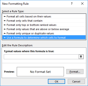
Step 2: Go to the “Home” tab → “Conditional Formatting” → “New Rule.”

Step 3: Click on the “New Rule.” It will open a separate dialog box. Then, select “Use a formula to determine which cell to format.”

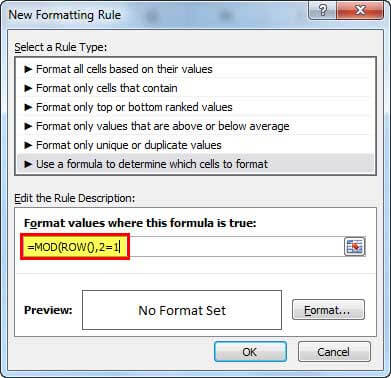
Step 4: In the formula section, we must mention = MOD (ROW (), 2) =1.

Step 5: Once the formula is inserted, click “Format.”

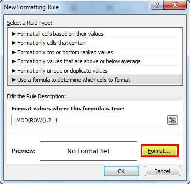
Step 6: Go to the “Fill” option and select the color as per choice.

Step 7: Click on the “OK.” It will highlight every alternate row.

How To Break Down The Formula

Let us break down and understand the formula =Mod (Row (), 2) = 1

The MOD function returns the remainder of the division calculation. For example, =MOD (3, 2) returns 1. When we divide the number 3 by 2, we will get 1 as the remainder. Similarly, the ROW function Excel will return the row number, and the number returned by the ROW function will be divided by 2. If the remaining number returned by the MOD function equals number 1, Excel may highlight the row by the mentioned color.

If the row number is divisible by 2, the remainder will be zero. On the other hand, if the row number is not divisible by 2, we will get the remainder equal to 1.
Similarly, if we want to highlight every third row, we must change the formula to =MOD (ROW (), 3) =1.
If we want to highlight every 2nd column, we can use =MOD (COLUMN (), 2) = 0.
We must use the formula. =MOD (COLUMN (), 2) =1, if we want to highlight every second column starting from the first column

Important Things To Note

If the data needs to be printed, we must use light colors to highlight it because dark colors may not show the fonts after printing.
If the header is selected while applying conditional formatting, it will be treated as the first row.
If we want to highlight every third row, we must divide the row by 3.
Similarly, we can apply this formatting for columns using the same formula.
We cannot change the color of the row once the conditional formatting is applied.

Frequently Asked Questions (FAQs)

1) What is an alternate way to Highlight Every Other Row In Excel?

Another alternate way to Highlight Every Other Row In Excel is by using the “Format Painter” option, as follows:
First, select a row which is already highlighted using the methods we learnt in this article.
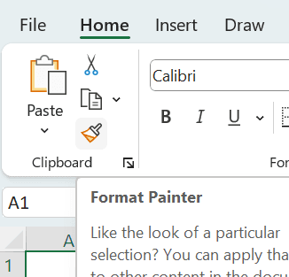
Next, select the “Home” tab → go to the “Clipboard” group → click the “Format Painter” option to copy the format, as shown below.

Finally, paste the copied format to the row which you want to format. Highlight Every Other Row In Excel is by using the “Format Painter” option

Repeat the steps for any rows you want to highlight.

2. What are different ways to Highlight Every Other Row In Excel?

We can highlight every other row or column in the following ways, namely:
1) Using Excel Table.
2) Using Conditional Formatting.
3) Using Custom Format.

3. Why is the highlighting of rows not working?

A few reasons why the highlighting of rows/columns may not work are,
• The new rule formula might not be rightly linked to the required cells.
• The proper rows or columns might not be selected.