Animation Chart in Excel

If the chart can convey the message so beautifully, how about adding animation to the chart? Animation? Yes, we can add animation to the charts that we create.

Animation charts require complete VBA knowledge, and mastering advanced VBA skills is not a walk in the park. It requires special dedication to learning those coding skills. Feeding your VBA animation chart is too much to digest at the moment. So, we will show you how to create animated charts in Excel without VBA coding.

For example, you have a GDP data set of four countries. Now, you need to animate them. Here, you may use a simple VBA Macro that will smoothly plot your values on the graph. Such an animated Excel chart is a powerful and eye-catching approach to grab the audience's attention and set your data in motion. Moreover, the animated effect widens the possibility of a chart telling a story on your behalf by bringing lives to the motionless GDP numbers.

Charts are like a beautiful garden in the city, and adding animation to the chart is the lovely flower in the park. Telling the story behind the data through animation goes a long way in holding on to the user's attention for a long time. Static charts are just enough to convey the message without any suspense, but adding animation to the chart is good enough to play with the audience's emotions.

Let us build the animation chart with Excel without the help of VBA coding.

For this animation, we have created the below data.

We will build an animated chart in Excel to show each quarter with this data.

The first thing we need to do is insert a column chart in excel for this data.

After inserting the chart, we need to insert "Option Button" from the Developer tab Excel.

Draw this “Option Button” on the chart.

Edit the text and enter it as “All Quarter.”

Right-click on the "Options Button" and choose "Format Control," or you can press Ctrl + 1 to open the "Format Control."

Select “Unchecked” and give “Cell link” to the A14 cell.

Press “OK.” We will have our first “Option Button” ready.

The above image shows that the “Option Button” is unchecked, and cell link A14 shows 0. However, if we check, the “Option Button” value in A14 becomes 1.

Like this, insert four more “Option Button” and name them “Q1,” “Q2,” “Q3,” and “Q4,” respectively.

Note: Give a cell link to the same cell, the A14 cell.

If the first “Option Button” is checked, then cell A14 value will change to 1. If the second “Option Button” is checked, then cell A14 value will be 2. For the third “Option Button,” it will change to 3.

We need to set up the data to show each quarter's sales separately. Create a replica of the data table to the right and add a new column as "Quarter."

In the "Quarter" column, we need to enter some formula to capture the data based on the "Option Button" selection we make.

Here, Jan, Feb, and Mar will be the first quarter, so we need to insert the below formula.

I have mentioned the IF formula in excel; it will reflect the data based on the "Option Button" selection. For example, if the Q1 option button is selected, it will reflect Jan, Feb, and Mar month numbers or the #NA value.

For Q2, from Apr to Jun, we need to change the logical condition from 2 to 3.

If the Q2 "Option Button" clicked, this formula shows numbers for this quarter. Similarly, now for Q3 and Q4, we need to enter a formula.

For Q3 enter the formula as =IF($A$14=4,E8,NA())

And for Q4 enter the formula as =IF($A$14=5,E9,NA())

We need to add data series to the existing chart with this rearranged data.

So, right-click on the chart and choose “Select Data.”

In the below window, press the "Add" button.

In the “Edit Series” window, choose "F1" for "Series Name," and for "Series Values," select "Quarter" column values.

Click on "OK," and we will have a chart like the below.

Select the column bars and press Ctrl+1 on the "Format Data Series" option.

In the “Format Data Series” window, make the series overlap as 100%.

Now, select the bar and make the color “light green” for all the bars.

And fill orange for " Series Quarter." We cannot see the impact immediately.

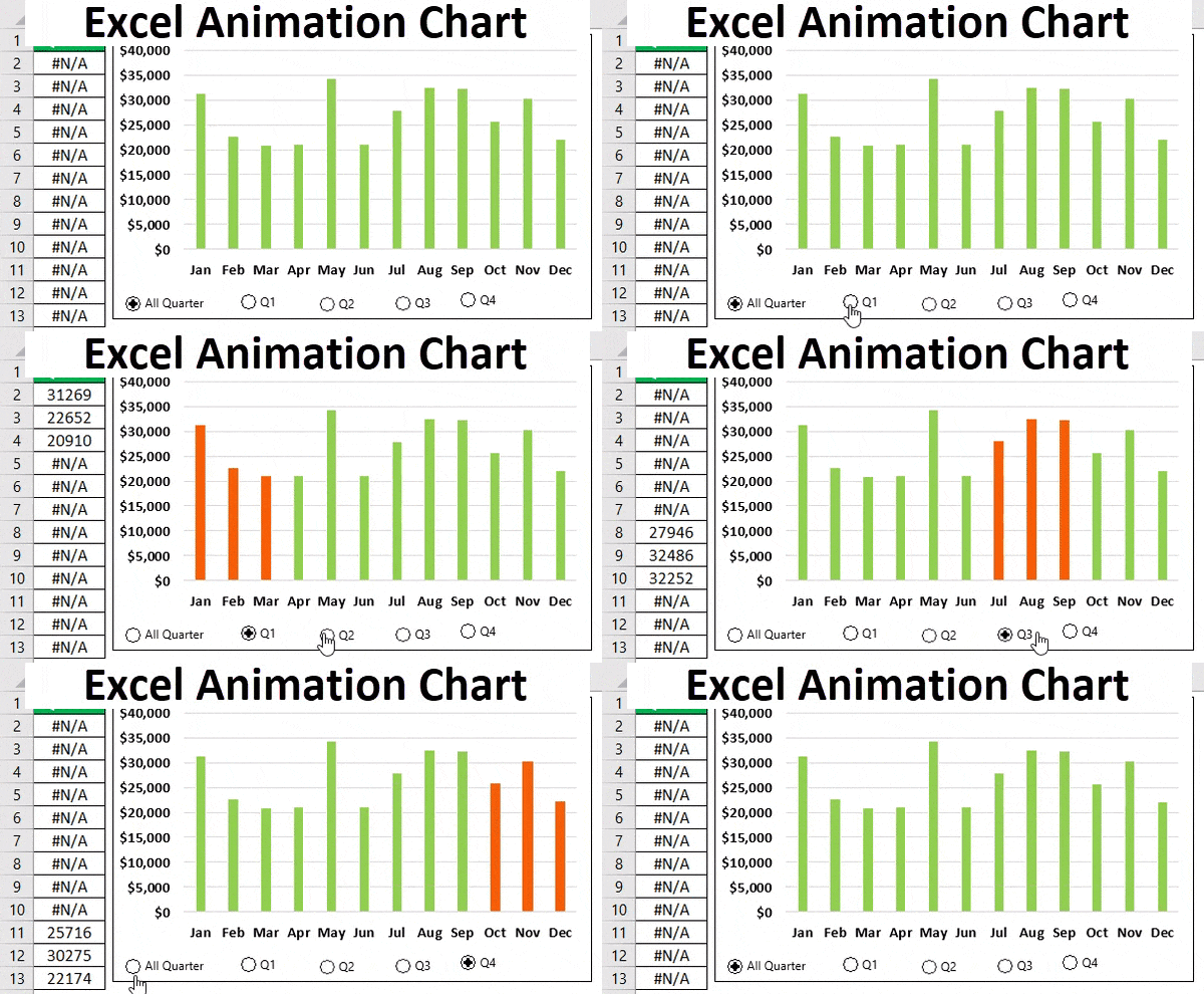
Now, we have completed the formatting.  Select the "Q1 Option Button" and see the magic.

We have selected the "Q1 Option Button”. In addition, "Q1" months data has been highlighted with orange.

Like this, without using VBA, we can create animation charts in Excel.

• Using VBA code is an advanced way of creating an animated chart but requires extensive coding.
• It is a simple example. We can create a wide variety of animation charts without the help of VBA.
• Using form controls in excel like checkbox, spin button, and options button, we can still create an animate chart without the help of VBA.