Funnel Chart In Excel

Last Updated :

21 Aug, 2024

Blog Author :

Edited by :

Reviewed by :

Table Of Contents

What Is Funnel Chart In Excel?

Funnel charts in Excel are similar to their name associated with them. It represents data behavior in every stage defined as the values decrease, thus making the shape of a funnel for the chart and the name of the funnel chart. This feature is only available in Microsoft office 2019 or the latest versions.

For example, consider the below table showing a company’s order details with no. of orders taken, confirmed orders, orders packed in warehouse, orders delivered without cancelling and ordered delivered with customer satisfaction.

Funnel Chart In Excel order process

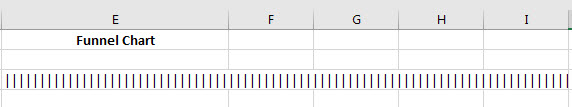
Among other methods, we can also use REPT function to create funnel chart in Excel as shown in the below image.

Funnel Chart In Excel order process - REPT function

Likewise, we can create funnel charts with simple steps. In this article, let us learn how to create funnel charts in Excel.

What Is Funnel Chart In Excel?
Funnel charts in Excel show data behavior as values decrease from stage to stage.
They resemble a funnel and are only available in Microsoft Office 2019 or later.
Funnel charts are helpful in sales, website trends, and order metrics.
Some of the charts are:
- Sales funnel charts show lost deals at each step.
- Website funnel charts show visitors to the "Home" page and those who downloaded or added products.
- Order funnel charts show initiated orders, canceled orders, returned orders and delivered orders to customers.

How To Create Funnel Chart In Excel?

Funnel charts in Excel, as the name suggests represents data in a funnel shaped chart. This resemblance helps users create visually appealing data with easy understanding of the data flows through the context.

Funnel Chart in Excel

Charts and other advanced tools in Excel are important for visually representing data and making it easier to identify patterns and trends. Learning Excel allows users to analyze complex data, automate tasks, and use advanced functions. Those looking to improve their data management skills using Excel can explore this Free Excel Course.

Let us learn how to create funnel chart in Excel with detailed examples.

Examples

Example #1

Suppose we have the following data for the order fulfillment process for an e-business organization.

funnel chart example 1.1

We will create an Excel funnel chart to display this data.

We need to use the REPT function in the following way. First, we can see that we have divided the value of B3 by 5 so that the size of the text does not exceed too much.
After inserting the function, we may find the output as follows.
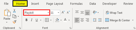
Since the output is not formatted in the way we want. So we need to change the font of the cell to "Playbill" using the "Font" text box in the "Font" Group in the "Home" tab.
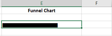
We want the line's color to be green and the alignment as a center. We will make necessary changes using the command available in the "Font" and the "Alignment" group in the "Home" tab.
We need to copy and paste the same formula and formatting on E3: E7.

Funnel chart Excel is ready. Whenever we change the value in the table, this chart will reflect dynamically.

Example #2

Suppose we have the same data as above, and we want to create a more attractive funnel chart.

funnel chart example 1.1

We will create the funnel chart using the 3-D 100% stacked column chart. The steps are as follows:

Step 1: We must first select the data range A2: B7.
Step 2: Then, click on the arrow located at the bottom right corner of the "Charts" group in the "Insert" tab.

funnel chart example 2.2

Step 3: Click on "All Charts," then choose "Column" from the list on the left, click on the "3-D 100% Stacked Column" chart, choose the second chart, and click on "OK."

funnel chart example 2.3

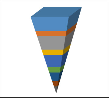
The chart will look as follows:

funnel chart example 2.5

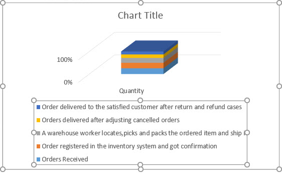
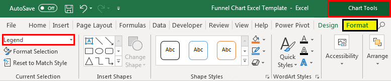
Step 4: Two new contextual tabs for chart tools (Design and Format) are opened when the chart is created. In the "Format" tab, we need to choose "Legend" from the list on the left side of the "Format" tab in the "Current Selection" group and press the "Delete" button on the keyboard to delete the legend.

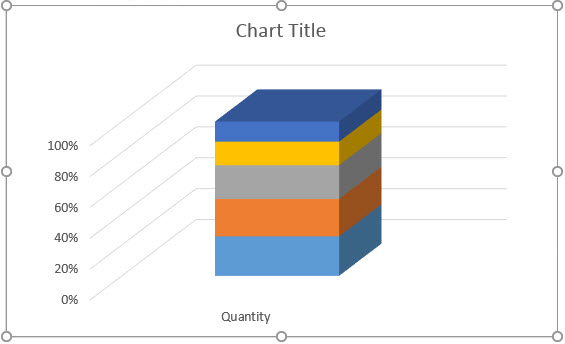
funnel chart example 2.4 funnel chart example 2.6

Step 5: In the same way, we will delete "Vertical (Value) Axis Major Gridlines," "Chart Title," and "Horizontal (Category) Axis."

funnel chart example 2.7

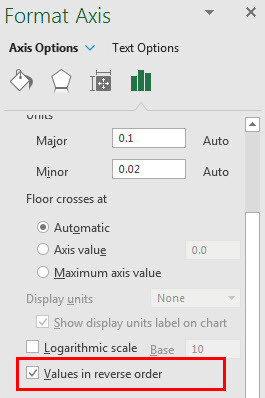
Step 6: Choose "Vertical (Value) Axis" from the list to select the axis in the chart. Now, choose "Format Axis" from the "Contextual" tab opened by right-clicking on the selection of the axis.

funnel chart example 2.8

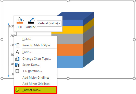
Step 7: Tick the checkbox for "Values in reverse order."

funnel chart example 2.9

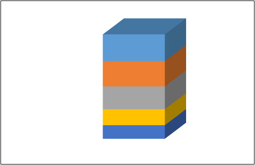
Step 8: Next, delete the "Vertical (Value) Axis" by selecting the same and pressing the "Delete" key.

funnel chart example 2.10

Step 9: Select any of the series from the list.

funnel chart example 2.11

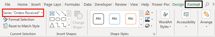
Step 10: Right-click on the series to get a "Contextual" menu and choose "Format Data Series" from the menu.

Format data series

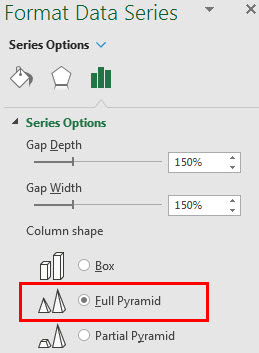
Step 11: Choose "Full Pyramid" from the list.

Format data series - Full Pyramid

Step 12: As we want to have some space in between the series, we can add rows for the same in the data as follows:

funnel chart example 2.14

Step 13: We need to change the data source for a chart using the "Select Data" command available in the "Data" group in the "Design" tab.

Design - Select Data

Step 14: Here, we must delete the selection and re-select the data using the range selector. Click on the "OK" button.

Select Data Source

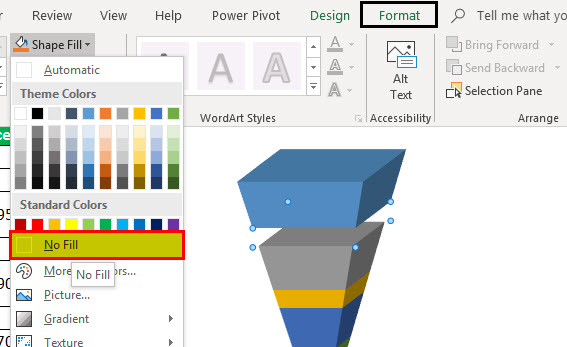
Step 15: As we can see, space, which we have specified in the data, is reflected in the chart in different colors. However, we want the space to be transparent.

funnel chart example 2.17

Step 16: To make the space transparent, we need to select the series by clicking on them and choosing "No Fill."

Format - No Fill Option

Now, we will follow the same for the other three series.

funnel chart example 2.19

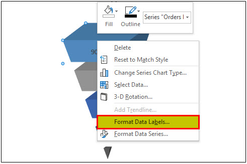
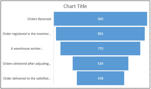
Step 17: We will add data labels and series names for all series by right-clicking on the series and choosing "Add Data Labels."

add data labels

Step 18: We can also add series names by formatting data labels.

add series names format data labels

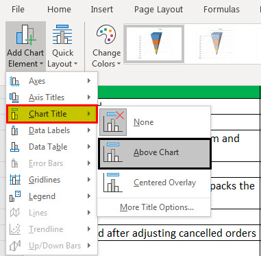
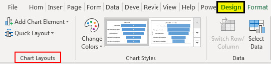
Step 19: We can add a chart title using the "Add Chart Element" command available in the "Chart Layouts" group in the "Design" tab.

chart tiltle - above chart

Now, our chart is ready.

example 2.24

Example #3

Suppose we have the same data as above.

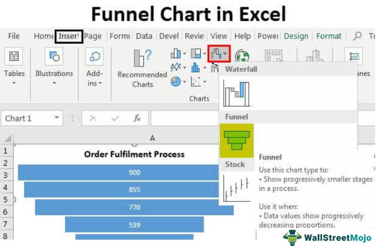
We can use the above two methods in the 2007, 2010, and 2016 versions of MS Excel, but the method discussed in this example is only available in Excel 2016, which is a funnel chart.

We can find the command in the "Charts" group in the "Insert" tab.

Insert tab - chart group

Now, to create the chart, we must follow the below steps:

Step 1: We must first select data A2: C7.
Step 2: Click on the "Funnel" command in the "Charts" group in the "Insert" tab.

example 3.2

Step 3: We will define the chart title and change the layout using the command available in the "Chart Layouts" group in "Design."

example 3.3

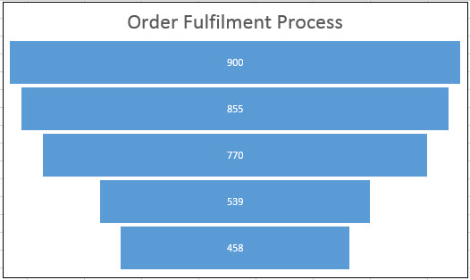
Now our chart is ready.

example 3.4

Uses Of Funnel Chart In Excel

The various places where we can use funnel chart are:

Sales Process: The funnel chart starts with the sales leads on top, then down to the qualified leads, then hot leads, and at last closed leads to the bottom. Any business loses several potential deals at each step in the sales process. The narrowing sections represent it as we move from the top area, the widest, to the bottom section, which is the narrowest section.
Website Visitor Trends: We can also use a funnel chart to display website visitor trends reflecting numbers of visitors who press the "Home" page at the extreme top with the widest area, and the other areas will be smaller, like the downloads or the people adding the product in the cart.
Order Fulfilment Funnel Chart: This chart could reflect initiated orders on top, canceled orders, returned orders, and at the extreme bottom, orders delivered to satisfied customers.

Important Things To Note

While taking the help of a funnel chart to display the data graphically, we must ensure that the process involves steps in which every previous step has a larger number than the next step.
It is because, the shape of the chart will look like a funnel.
One must create a funnel chart with decreasing values for each step to form a funnel shape.

Frequently Asked Questions

1. How to rotate funnel chart in Excel?

To rotate a pyramid, right-click on it, select "3-D Rotation" from the fly-out menu, and adjust the X and Y Rotation to 0o in the 3-D Rotation section of the Format Chart Area pane.

2. How do I add labels to a funnel chart in Excel?

For example, consider the below table and funnel chart.

Funnel Chart In Excel order process example

To add data labels to a chart, navigate to the "Chart Design tab," select "Data Labels," and choose a location for the label, adjusting depending on the chart type. Now, the chart will appear as shown in the below image.

Funnel Chart In Excel - order process example 2

3. How do I edit a funnel chart in Excel?

Insert data into a stacked bar chart, right-click on it, select 'Change Chart Type,' and choose "Funnel Chart." Customize the chart by going to the 'Design' and 'Format' tabs on the Excel ribbon.